Determine the highest (or lowest) elevation point within a polygon with SAGA GIS

The example workflow described here can be used to locate possible sites for locating radio towers or something similar. Along the way, it also illustrates how to use SAGA GIS to create a buffer zone around a point, how to use the buffer zone as a polygon to find the location of the maximum elevation on a DEM, and how to sort attribute tables.

Load in a DEM grid layer and a point shape layer

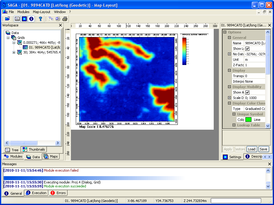
1. Start up SAGA GIS and load in and display a DEM grid layer, e.g. ground.asc.
2. Load in and display a point shape file, e.g. bufferPoint.shp in the same map window.
   
   The grid layer and point shape layer are loaded.
   

Create the buffer zone

1.  Select Modules | Shapes | Tools | Shapes Buffer.
   
   The Shapes Buffer dialog box appears.
   
2. Click the Shapes row and select the point shape layer e.g. 01.bufferPoint.
3. In the Buffer Distance (Fixed) field, type in a distance, e.g. 100.
   
   
4. Click Okay.
   
   The buffer polygon is created around the point.
   

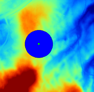
Generating the highest (and lowest) elevations for the entire DEM grid layer

1. Select Modules | Shapes | Grid | Local Minima and Maxima.
   
   The Local Minima and Maxima dialog box appears.
   
2. Click the Grid system row and choose the DEM grid system, e.g. 1;684x684y;312480x5195216y.
3. Click the Grid row and choose the input DEM grid layer, e.g. 01.ground.
   
   
4. Click Okay.
   
   The local minima and maxima point shapes for the entire DEM grid layer are created.
   

Finding only the local maxima point shapes within the buffer

1. Select Modules | Shapes | Construction | Cut Shapes Layer.
   
   The Cut Shapes Layer dialog box appears.
   
2. Click the Shapes row. Then click the browse [...] button.
   
   The Shapes dialog box appears.
   
3. Select the local maxima point shape layer, e.g. 03.ground[Local Maxima] on the left list. Click the >> button.
   
   The selected layer is shifted to the right list.
4. Click Okay.
5. Ensure the Method is completely contained. Click the Options Extent row and select polygons.
   
   
6. Click Okay.
   
   Processing messages appear.
   
   
   The Polygons dialog box appears.
   
7. Click the Polygons row and choose the buffer shape layer, e.g. 01.bufferPoint[Buffer].
   
   
8. Click Okay.
   
   The local maxima points within the buffer is generated.
   

Locating the maximum point within the buffer

1. In the Workspace pane, mouse right click on the local maximum points within the buffer layer, e.g. 04.ground[Local Maxima][Cut].
   
   A pop up menu appears.
   
2. Select Attributes |  Show Table.
   
   The attribute table appears.
3. Select Window | Tile Horizontally.
   
   
4. In the attribute window, double click the Z column title header to sort the records so that the maximum Z value is the first row.
5. Select the first row (which has the maximum elevation).
   
   The corresponding point on the map window is highlighted.
   

Import GeoMedia Access Warehouse features into gvSIG

I recently installed and tried out the open source Java GIS application gvSIG OADE version 2010 from Oxford Archaeology along with a free extmdb extension to read features from a GeoMedia Access warehouse from the Google Code project site. I found the process to create a gvSIG project and import GeoMedia features to be relatively straightforward. Maybe the one thing to take note of is that the loaded GeoMedia features are temporary in nature only and must be saved permanently as gvSIG compatible formats e.g. Shape file.

In this example, I am going to import in a feature from the GeoMedia sample warehouse USSampleData.mdb file, which uses the Albers Equal Area coordinate system.

Create a new gvSIG project and assign a coordinate system

1. Select Start | All Programs | gvSIG OA Digital Edition 2010 | gvSIG OA Digital Edition 2010.
   
   The gvSIG OADE 2010:Untitled application appears.
   
   
2. In the Project manager window, click View | New.
   
   An Untitled-0 view is created and added to the View list box.
   
   
3. In the View group box, select Untitled-0. Click Properties.
   
   The View properties dialog box appears.
   
   
4. Click the Current projection button.
   
   The Spatial Reference System (SRS) dialog box appears.
   
   
5. Click the Type combo box. Choose a suitable type e.g. ESRI.
6. Toggle on By name.
   
   
   
7. In the Search criteria field, type in Albers. Click Search.
   
   A list of matching results appear.
   
   
8. Select USA_Contiguous_Albers_Equal_Area. Click OK.
   
   
   
9. Click OK again.
10. In the View group box, click Open.
    
    The View:Untitled-0 window is opened.
    

Import GeoMedia features

1. Select View | Add Layer.
   
   The Add Layer dialog box appears.
   
   
2. Click the MDB tab.
   
   
   
3. Click the Search button.
   
   The Open dialog box appears.
   
   
4. Browse and select a GeoMedia MDB file e.g. C:\Warehouses\USSampleData.mdb. Click Open.
   
   The GeoMedia feature names are displayed in the Feature Classes grid.
   
   
   
   
5. Toggle on the feature(s) to add, e.g. States. Click OK.
   
   Processing messages appear and the selected features are imported.
   
   
6. Close the message box.
   
   The imported features are displayed in the view.
   

Export GeoMedia feature(s)

1. In the View legend, click the feature name to be exported e.g. States.
   
2. Select Layer | Export To | Shapefile.
   
   The Save dialog box appears.
   
   
3. Type in the file name e.g. States. Click Save.
   
   Processing messages appear.
    
   
4. Click Yes.
   
   The exported shapefile is added as a layer to the view.

Remove the GeoMedia warehouse from the view

1. In the View legend, mouse right click on the warehouse name e.g. USSampleData.
   
   A pop up menu appears.
   
   
2. Choose Delete.
   
   A prompt appears.
   
   
3. Click Yes.
   
   The GeoMedia warehouse is removed from the view.

Save the gvSIG project

1. Select File | Save project.
   
   The Save project dialog box appears.
   
   
2. Type in a file name, e.g. geomedia.gvp. Click Save.
   
   The project is saved.

Export a map layout to KML from SAGA GIS

The contents of the Map Layout window in SAGA GIS can be exported as KML files and displayed in Google Earth. There is a catch, however: SAGA GIS will always create the KML files but it will not do an automatic coordinate system conversion to Geodetic Lat/Long.

Before creating the Map Layout window for export, all the data layers must be projected into the geographic Lat/Long coordinate system first. See my previous post on how to do reprojection.

The steps to export out as KML are below, assuming all the data layers are already in geographic Lat/Long.

1. Start up SAGA GIS. Load in one or more grid layers and display them in one map window.
   
   
2. Select Map | Show Print Layout.
   
   The Map Layout window appears.
   
3. In the Workspace pane, activate the Map tab.
   
   
4. In the Maps tree, mouse right click on the map name.
   
   A pop up menu appears.
   
5. Choose Save as Image.
   
   The Save As Image dialog box appears.
   
6. Specify an output file name and type, e.g. 9894CATD and PNG. Click Save.
   
   The Save Map as Image dialog box appears.
   
7. Toggle Save KML file on. Click Okay.
   
   The KML file is created.
   

The screenshot below shows how the KML file looks like in Google Earth. 

Reprojecting a grid file in SAGA GIS to a new coordinate system

There are SAGA GIS modules to perform re-projection of grid and shape layers from one coordinate system to another coordinate system. The workflow is quite straightforward. The only inconvenience is having to define the source and destination coordinate system each time you run the projection module.

Below is an example of projecting a grid layer from UTM Zone 16, NAD83 datum to geodetic latitude and longitude.

1. Start up SAGA GIS. Load in a grid layer.
2. Select Modules | Projection | Grid | Proj.4 (Dialog, Grid).
   
   The Proj.4 (Dialog, Grid) dialog box appears.
   
   
3. Select the Source Projection Parameters row. Click the [...] button.
   
   The Source Projection Parameters dialog box appears.
   
   
4. Select the Projection Type row. Choose a projection e.g. Universal Transverse Mercator (UTM).
5. Select the Predefined Datum row. Choose a datum e.g. [NAD83] North_American_Datum_1983.
6. Click Okay.
7. Select the Grid system row. Choose the grid layer's system e.g. 30;384x464y;545765x3831410y.
8. Select the Source row. Choose the grid layer name e.g. 01.9894CATD.
9. Select the Target Projection Parameters row. Click the [...] button.
   
   The Target Projection Parameters dialog box appears.
   
   
10. Select the Projection type row. Choose the destination projection e.g. Lat/long(Geodetic).
    
11. Select the Predefined Datum row. Choose the datum e.g. [WGS84]. Click OK.
    
    
    
12. Click OK.
    
    The Universal Transverse Mercator (UTM) dialog box appears.
    
    
13. In the Zone field, type in 16. Click Okay.
    
    The User Defined Grid dialog box appears.
    
    
14. If necessary, change the values. Click Okay.
    
    A new grid layer is created with the target coordinate system.