Detect changes between 2 polygon layers in gvSIG

gvSIG can be used to identify the spatial changes between two polygon vector layers. This can be done by using the Geoprocessing tools' Analysis Overlay difference function. An illustration of this is described below using the scenario of identifying the new vegetation growth and the loss of vegetation cover between a period of time.

Identify new vegetation growth

1. Start gvSIG OADE. Open a map view. Load and display two polygon layers e.g. vegetation2001.shp and vegetation2011.shp.
   
   
2. Select View | Geoprocessing tools.
   
   The Geoprocessing tools dialog appears.
   
3. Expand the nodes Geoprocessing tools | Analysis | Overlay. Select Difference. Click Open Tool.
   
   The Analysis tools dialog box appears.
   
4. In the Input layer field, choose vegetation2011.
5. In the Overlay layer field, choose vegetation2001.
6. In the Output layer field, type in the output file name, e.g. C:\temp\new_growth.shp.
7. Click OK.
   
   The polygons representing the new vegetation growth is created.
   

Identify the loss in vegetation cover

1. If the Geoprocessing tools dialog is not opened, then select View | Geoprocessing tools.
   
   The Geoprocessing tools dialog is displayed.
2. Expand the nodes Geoprocessing tools | Analysis | Overlay. Select Difference.
3. Click Open tool.
   
   The Analysis tools dialog box appears.
   
4. In the Input layer field, choose vegetation2001.
5. In the Overlay layer field, choose vegetation2011.
6. In the Output layer field, type in the output file name e.g. C:\temp\loss_of_vegetation.shp.
7. Click OK.
   
   The polygons representing the loss in vegetation cover are created.
   

Use gvSIG to create Voronoi or Thiessen polygons

A GIS software such as gvSIG can help marketers to create polygons representing regional areas of coverage for their companies' branch offices if none are available. All that is required are the points representing the offices and perhaps a polygon representing the overall area of coverage e.g. the State boundary.

The basic steps to create the regional areas are simply the following:

1. Generate Voronoi or Thiessen polygons from the points
2. Mask away the extra parts of the Voronoi polygons from the area of coverage polygon

For a detailed explanation of Voronoi or Thiessen polygons, visit the Wikipedia site http://en.wikipedia.org/wiki/Voronoi_diagram.

The example below illustrates how to generate the Voronoi polygons of cities in the state of Montana.

1. Start gvSIG OADE. Load and display the cities and the state boundary polygon in a map view.
   
   
   
2. Select View | Geoprocessing tools.
   
   The Geoprocessing tools dialog box appears.
   
   
3. Expand the Geoprocessing tools | Analysis | Computational geometry nodes. Double click Voronoi/Delaunay.
   
   The Analysis tools dialog box appears.
   
   
4. In the Input layer field, choose the points layer e.g. cities_in_montana.shp.
   
5. Toggle on Voronoi(Thiessen) polygons.
   
6. In the Output layer field, click Choose. In the Save dialog, type in the output layer name e.g. c:\temp\voronoi.shp. Click Save. Click OK.
   
   The polygons are generated.
    
   
7. If the Geoprocessing tools dialog box is closed, select View | Geoprocessing tools.
   
   
   
8. Expand the Geoprocessing tools | Analysis | Overlay nodes. Double click on Intersection.
   
   The Analysis tools dialog box appears.
   
   
9. In the Input layer field, choose the newly created Voronoi polygons layer e.g. voronoi.shp.
   
10. In the Overlay layer field, choose the overall area of coverage polygon layer e.g. montana.shp.
    
11. In the Output layer field, click Choose. In the Save dialog box, type in the output layer name e.g. c:\temp\cities_coverage_pol.shp. Click Save.
    
12. Click Ok.
    
    The final regional area polygons are created and nicely masked.
    

Example of using gvSIG'S Modeler

gvSIG's Modeler function can be used to create reusable models of processes that can be applied on geographical vector and raster data layers. For example, if you need to periodically generate centroids and calculate the centroid coordinates from polygon vector layers, then it may be worthwhile to use the Modeler. Once you have a model of the processes created, it is a simple matter to reload the model and run it.

The models are almost similar to programming scripts except that you don't need to be a developer to create them. You simply use a graphical user interface to point and click to define the model. The example below shows how easy it is to create the model with the Modeler.

Create a New Model

1. Start gvSIG OADE 2010. Load and display a vector polygon layer e.g. C:\data\States.shp.
   
   
2. Click the Modeler   icon in the tool bar.
   
   The Modeler dialog box appears.
   
3. In the Inputs tree, double click on Vector layer.
   
   A dialog box appears.
   
4. In the combo box, choose Polygons. Click OK.
   
   The Vector layer1 icon appears in the Modeler dialog box.
5. Click the Procedures tab. Under the Procedures | Algorithms tree, expand the Tools for polygon layers node. Double click Centroids.
   
   A dialog box pops up.
   
6. Click OK.
   
   A Centroids icon appears connected to the Vector layer1 icon in the Modeler dialog box.
7. Under the Procedures | Algorithms tree, expand the Tools for point layers node. Double click Add coordinates to points.
   
   A dialog box appears.
   
   
   
8. Toggle on Keep as final result.
9. Optional. In the Name field, type in the output point layer name.
10. Click OK.
    
    The Add coordinates to points icon is displayed connected to the Centroids icon in the Modeler dialog box.
    
    Note: To save the model, click Save and specify the output file path and name. 

Running a Model

1. Click Run.
   
   The [Model] dialog box appears.
   
2. In the Inputs Vector layer field, choose a polygon layer e.g. States.shp.
3. Optional. In the Outputs field, type in a new output Shape file path and name.
4. Click OK.
   
   The processes defined by the model is executed and the output layer(s) is created.
   
5. Close the Run model dialog box.
6. Optional. To review the centroid point coordinates, select the newly created layer in the legend and choose Layer | Show attribute table.
   
   The attribute table appears as shown below. Note the two newly created X and Y attribute fields.
   

Using gvSIG's Geographic Transformation on a raster file

gvSIG has a Photoshop-like tool that can be used to perform geometric transformations on raster files. Transformations such as translation, rotation, scaling, and skewing can be applied interactively to a raster file. The example below illustrates the Geographic Transformation command.

Start the Transformation command

1. Run gvSIG OADE 2010. Load and display a raster file.
   
   
   
   
2. In the toolbar, locate the Geographic transformation icon as shown below.
   
   
   
   
3. Then locate and click the Transformation icon as shown below.
   
    
   
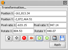
   The Transformation dialog box appears.
   
   
   Note: the raster layer can be transformed either by changing the values in the Transformation dialog box or by graphically adjusting the image in the map view.
   
4. In the Transformation dialog box, click the Center raster layer in view icon.
   
   The raster layer is scaled, moved and centered in the map view.
   
   
   Moving the raster image

1. In the map view. move the cursor to the middle of the raster image.
   
   The cursor becomes a hand.
   
2. Press down the mouse left button and drag the image.
   
   The raster image is moved to another location.
   
   

Skew the image in the Y-axis direction

1. Move the cursor to the vertical sides of the raster image.
   
   The cursor changes to an arrow with a Y label.
   
2. Press down the left mouse button and drag the image along the Y axis.
   
   The image is skewed in the Y-axis direction.
   
   

Skew the raster image in the X-axis direction

1. Move the cursor to the horizontal sides of the raster image.
   
   The cursor changes to an arrow with the label X.
   
2. Press down the left mouse button and drag the image in the X-axis direction.
   
   The raster image becomes skewed in the X-axis direction.
   

Rotate the raster image

1. Move the cursor to any corners of the raster image.
   
   The cursor changes to a rounded arrow.
   
2. Press down the left mouse button and drag the image around the corner.
   
   The raster image is rotated.
   

Resize the raster image

1. Move the cursor along the sides and corners of the raster image.
   
   The cursor changes to a two-headed arrow.
   
2. Press down the left mouse button and drag the image inwards or outwards.
   
   The raster image is resized.
   

Save the transformation

1. In the Transformation dialog box, click the Save transformation icon.
   
   The message appears.
   
   
   
2. Click Yes.
   
   The adjustments are saved.

Georereference a raster file in gvSIG

There is a function in gvSIG that you can use to georeference any raster images such as scanned images, or photos. The gvSIG georeference function will create world files and other georeferencing metadata information that can be used only with gvSIG apparently. The georeference function has a field to specify the output georeference file but the file is never created. If you want to register raster images for use in gvSIG, then the example below demonstrates the procedure.

Load reference layers and setup the georeferencing views

1. Start gvSIG. Load and display any geographic features that can be used to aid the georeferencing.
   
   
2. Select Tools | Georeferencing.
   
   The Georeferencing dialog box appears.
   
   
3. If necessary, toggle on With reference map. Choose a Map view e.g. Untitled - 0.
   
4. In the File to georeference field, click Select.
   
   The Open dialog box appears.
   
   
5. Browse to the raster file e.g. C:\Temp\georef\spiritlakegeology.sid. Click Open.
   
6. If necessary, toggle on Affine transformation.
   
7. Click Accept.
   
   The Georeferencing views, Zoomed views, and Ground control points (GCP) windows appear.
   

 Add Ground Control Points

1. In the Ground control points (GCP) window, click the New * icon.
   
   A new row is added to the GCP list.
   
   
2. Use the Zoom icons on the right side of the right Georeferencing view to manipulate the corner of the raster image into the central red box.
   
   
   
   Note: I used the Zoom to select area to zoom in closer to the corner; then the Move image icon to move the corner into the red box.
   
   
3. In the right Zoomed view, click on the raster image corner.
   
   A numbered GCP cross is displayed at the clicked location.
   
   
4. Use the Zoom icons on the right side of the left Georeferencing view to manipulate the corresponding point of the referencing layers to the central red box.
   
    
5. In the left Zoomed view, click on the corresponding corner point.
   
   A numbered GCP cross is displayed at the clicked point.
   
6. Repeat the previous steps 1 to 5 to add in at least 3 GCP points for (Affine transformation).
   
   
   
   Note: If the RMS values in the Ground control points (GCP) window is very large, it may be necessary to edit the control points. 

Applying the transformation

1. In the Ground control points (GCP) window, click the Apply icon.
   
   The raster image is warped into the left Georeferencing view.
   
   
   
2. In the Ground control points (GCP) window, click the Exit (and save) icon. Click Yes to the prompts.
   
   The following prompts appear.
   
   
   
   
   The raster image is warped and displayed in the map view.