Digitizing New Lines with Global Mapper

I have always used Global Mapper mostly as a viewer and converter for GIS files. Recently I tried out the digitizing commands on Global Mapper 10 and 11 and I found them to be surprisingly competent and powerful to create and edit point, line, and polygon vector features. Version 11 has some improvements over Version 10 - the most notable one being the new Digitizing toolbar, which is not available on the older version.

To use the digitizing functions, you have to enter digitizing mode by clicking the Digitizer Tool button in Global Mapper.

In Global Mapper 11, the Digitizer Toolbar will appear as shown below.

And the screen cursor would change to a cross hair with a EDIT label at the bottom.

A right click in the map display would bring up a context menu as shown below.

If I want to create a new line feature, then I would choose Create New Line Feature in the pop up context menu. The screen cursor label would change to the string "LINE".

As shown in the screen shot below, I can Left-click with the mouse button to place consecutive points of the line feature.

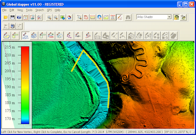
To complete the placement of the new line feature, Right-click with the mouse button. Then the Modify Feature Info dialog box will pop up.

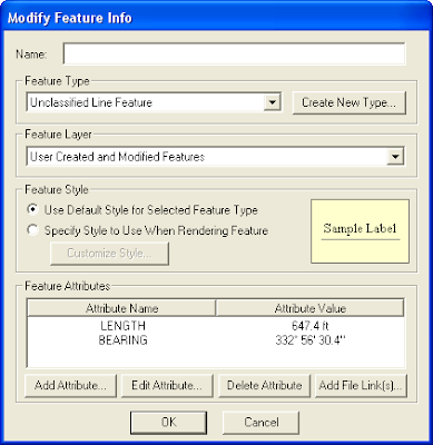
In the Feature Type drop down list, you can choose any pre-defined feature type e.g. River, Unknown Length. Or create your own type by clicking the Create New Type button.

You can choose to place the new line on an existing layer or a new layer by choosing <Create New Layer for Feature> in the Feature Layer drop down list.

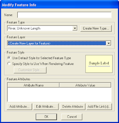
After you click OK, it will prompt you for the new layer name. Just type in a new name e.g. Rivers and click OK.

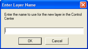
Your new line feature is created and placed in the layer you want.

Lidar LAS file conversion to Tiff using FME

I tried out using Safe FME to convert a Lidar LAS file to a grayscale TIFF image file and I was reasonably successful doing it. I'm not quite completely happy with it ( for instance, it would be more correct to filter out all returns except the first return) but here are the steps that I took.

1. From the FME Workbench, create a translation using the translation wizard. Choose ASFPRS Lidar Data Exchange Format (LAS) as the source dataset. Click Next.
   
   
   
   
2. When prompted to specify the location of the source data, browse and select the input LAS file, e.g. Serpent Mound LAS Data.las. Click Next.
   
   
   
   
3. When prompted to Select Destination Format, choose GeoTIFF (Georeferenced Tagged Image File Format). Click Next.
   
   
   
   
4. In the Select Feature Types dialog box, toggle off header and variable_length_header feature types if you like because we are only interested in the point feature type. Click OK.
   
   
   
   
5. Within the workbench, drag and drop the transformers ExpressionEvaluator, Concatenator, and ImageRasterizer onto the workbench. Connect them up with the source and destination datasets as shown in the figure below.
   
   
   
   
6. Open up the ExpressionEvaluator transformer's Properties. In the Expression field, type in @Value(Intensity). Click OK.
   
   Note: the output from this transformer is the attribute _result by default.
   
   
   
   
7. Open up the Concatenator transformer's Settings dialog box. Form the string "_result, _result, _result" in the Concatenated Items box. In the Destination Attribute field, change the text to fme_color. Click OK.
   
   Note: in this step, we are forming the rgb string. Since intensity images are grayscale, we simply repeat the same intensity value in the red, green, and blue parts of the output fme_color string.
   
   
   
   
8. Open up the ImageRasterizer transformer's Parameters dialog box.
   
   
   
   
9. In the Rows/Columns or Cell Size field, choose CellSize.
   
   
10. In the X Cell Spacing and Y Cell Spacing fields, type in the desired TIFF pixel size e.g. 1 m.
    
    
11. In the Interpretation Type field, choose Gray8. Click OK.
    
    
12. Run the translation.
    
    The intensity image is created from the source LAS file.
    
    
    The resultant intensity image isn't too bad but as I said earlier, the process can be improved. Maybe next time...

Select and update feature attributes in GeoMedia

In GeoMedia, there is a useful function to select one or more geographical features and update their attributes but it is hidden away under some pulldown menus. Sometimes it is easier for users to use the Selection tool and simply point and click to select features for updating.

In this example, I want to update the STATE_NAME attribute of the Counties feature to e.g. Alabama. Here are the steps:

1. In GeoMedia, click the Selection Tool button.
   
   
   
   
2. In the map view, click on one or more Counties feature.
   
   The features are selected (in green color).
   
   Note: Press CTRL + click to add more features to the selection set.
   
   
3. Select Edit > Attribute > Update Attributes.
   
   
   
   The Update Attributes dialog box appears.
   
   
   
4. In the Update Features In box, expand the Select Set node. Expand the Warehouse node. Select the Feature name, in this example, it is Counties.
   
   The attributes of the selected feature are displayed in the Attributes to Update box.
   
   
5. In the Attributes to Update box, scroll to the attribute(s) you want to update e.g. STATE_NAME and type in the new value e.g. Alabama.
   
   At this point, the Update Attributes dialog box may look like this.
   
   
   
6. Click Apply.
   
   The selected features are updated with the new attribute values.
   
   
7. Close the dialog box.

QC digital terrain model for isolated spikes with color gradients

A quick way to find out whether your digital terrain model file has isolated high points or spikes is to display the terrain model with a color gradient from blue to red as shown in the Global Mapper screenshot below.

In this example, the terrain surface is mostly shaded in blue tones. That is a good indication that there are some elevation spikes somewhere in your terrain model.

A screenshot of a digital terrain model file with no high points is shown below. A good terrain surface is shaded evenly with the colors nicely balanced from blue to red as you go from lower elevations to higher elevations.

This is one way to quickly check your digital elevation models for the presence of isolated elevation spikes.

Some useful Linux remote commands (to me)

Sometimes I need to dial in to a remote computer running Linux to run some Linux batch processing commands which may take a while to complete. Normally, once you logged out from the remote computer, the processes that you started during the remote login session will be terminated. There is a modifier command that you can use to make sure the processes keep on running even after you logged out.

The modifier command is nohup, which stands for "no hang up". This is how it is used:

$ nohup your_long_process_command &

where your_long_process_command is obviously your long process command name.

Any processing messages printed out by your process would be rerouted to the text file nohup.out.

You can now logged out from the remote computer.

The next time you dial in to check on the status of your process, you can either review the nohup.out file with a text editor or you can run the following command to see whether it is still running in the process list.

$ ps -ef | grep your_long_process_command

If it returns a process list number, then it is still running.

Quickly attach xls/csv/dbf files in GeoMedia

GeoMedia allows you to connect to text files via the Text File Data Server connection, which requires you to define a text file server definition file. Although this method is powerful and flexible, it is not easy for users to grasp. There is an alternative quick and easy way in GeoMedia to attach and display the same text files via the Attach as Feature Table function. This function also allows you to display Excel spreadsheets (*.xls) and Dbase files (*.dbf), in addition to CSV text files (*.txt, *.csv). Here are the steps.

In this example, I want to attach the CSV text file shown below in a text editor. It has the standard header in the first line and the comma separated records below that.

1. In GeoMedia, connect to a Access read/write database.
   
   
2. Select Warehouse > Feature Class Definition.
   
   The Feature Class Definition dialog box appears.
   
   
   
3. In the Feature Classes box, click a Access read/write connection e.g. tmp. Click Attach.
   
   The Attach dialog box appears.
   
   
   
4. In the Type combo box, choose the type of file you want to attach, e.g. Text. Click Browse.
   
   The Open dialog box appears.
   
   
   
5. Browse and select the file you want to attach, e.g. gps.csv. Click Open.
   
   The Attach dialog box is updated with the selected file.
   
   
   
6. If you like, change the default name of the target table. Click OK.
   
   The attach feature table is appended to the Access connection.
   
   
   
7. Click Close.

From now on, you can display and manipulate the records in the attached file within GeoMedia. For instance, you can select Window > Data Window and display the contents of the file as shown below.

Create a GeoTiff image from shape file using FME

I thought I'd try out using FME to create GeoTiff images from vector geometries. It is actually quite straightforward and the trick is to make sure that the fme_color attribute is set to some rgb value either explicitly or through the PenColorSetter transformer. In this simple example, I convert a polygon geometry shape file to a GeoTiff image file.

1. Using the FME Workbench, create a Shape file to GeoTiff translation workflow as shown in the figure below. Add in the PenColorSetter and ImageRasterizer transformers and connect them up accordingly.
   
   
   
   
2. Open up the PenColorSetter Parameters. Define a Pen Color, e.g. red.
   
   
   
   
3. Open up the ImageRasterizer Parameters.
   
   
4. In the Rows/Columns or Cell Size field, choose RowsColumns (if you want to set the GeoTiff image file dimensions by cell size, then choose CellSize and define the X and Y Cell Spacing).
   
   
5. In the Number of columns field, enter the horizontal pixel dimensions e.g. 1000.
   
   
6. In the Number of rows field, enter the vertical pixel dimensions e.g. 800.
   
   The ImageRasterizer Parameters may look like this at this point.
   
   
   
7. Close the ImageRasterizer Parameters dialog box.
   
   
8. The source and destination coordinate system should be set if you want to create a geo-referenced GeoTiff image file. In the Navigator pane, define the source dataset coordinate system, e.g. LL84 for geographic WGS84.
   
   
   
9. In the Navigation pane's destination coordinate system parameter, define the destination GeoTiff dataset's coordinate system, e.g. LL84.
   
   
10. Run the translation.
    
    The GeoTiff image file is generated.

The resultant GeoTiff image file can be opened up in any GIS application software like GeoMedia or Global Mapper as shown below.