Remove noisy spikes from LiDAR data using SAGA GIS and SRTM data

LiDAR data collected from the field contains noise in the form of spikes or zingers (extremely high or low points) and/or clouds. Typically these erroneous points are reclassified as noise from the point cloud by using high-low filters, median filters or other statistical methods. An example is shown in the screenshot below.


I have in mind using the globally available Shuttle Radar Topography Mission (SRTM) data to form an envelope to filter away the extreme noise points using SAGA GIS. SRTM data can be downloaded from http://www2.jpl.nasa.gov/srtm/.

From the SRTM elevation data, a height value can be added and subtracted to form a volume envelope. Any LiDAR points inside the envelope are valid points while any points outside the envelope are noise. The following illustrates a possible workflow.

Load and reproject an SRTM tile to match the LiDAR data

1. Start SAGA GIS.
2. Select Modules | File | Grid | Import | Import USGS SRTM Grid.
   
   The Import USGS SRTM Grid dialog appears.
   
   
3. Click the Files field. Then click the browse [...] button. Browse and select an SRTM file e.g. N39W084.hgt. Click Open. Click Okay.
   
   The SRTM data is loaded.
   
   Note: the SRTM data is in a geographical latitude-longitude coordinate system while the LiDAR data is in a projected coordinate system e.g. UTM 17 North.
   
4. Select Modules | Projection | Coordinate Transformation (Grid).
   
   The Coordinate Transformation (Grid) dialog box appears.
   
   
5. In the EPSG Code | Projected Coordinate Systems field, choose a coordinate system e.g. WGS 84 / UTM zone 17N.
6. In the Data Objects | Grid system field, choose the SRTM grid system e.g. 0.000833; 1201x 1201y; -84x 39y.
7. In the Data Objects | Grid system | source field, choose the SRTM grid layer e.g. 01.N39W084.
   
   
   
8. Click Okay.
   
   The User Defined Grid dialog box appears.
   
   
   
9. Click Okay.
   
   The SRTM grid is reprojected into UTM 17 North.
   
   Note: there are now two SRTM grid layers with the same name. For clarity, we shall remove the first SRTM grid layer.
   
10. In the Data tab of the Workspace pane, select the first SRTM grid layer e.g. 01. N39W084.
    
11. Press the mouse right click button. In the pop up menu, select Close.
    
    
    
12. Click Yes and Okay.
    
    The original SRTM grid layer is removed.

Load the LiDAR LAS file

1. Select Modules | File | Shapes | Import | Import LAS Files.
   
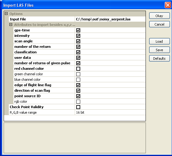
   The Import LAS Files dialog box appears.
   
2. Click the Input file field. Click the browse [...] button and select and open a LiDAR LAS file .e.g. noisy_serpent.las.
   
3. In the Attributes to import besides x,y,z list, toggle on all the attributes you want to retain.
   
   
   
4. Click Okay.
   
   The LAS file is loaded as a PointCloud.
   

Assign the SRTM elevations to each LiDAR point

1. Select Modules | Shapes | Grid | Grid Values | Add Grid Values to Shapes.
   
   The Add Grid Values to Shapes dialog box appears.
   
2. In the Shapes field, choose the LiDAR point cloud layer e.g. 01. noisy_serpent.
   
3. In the Grids field, click the [...] button. Choose the reprojected SRTM grid layer e.g. 01.N39W084.
   
   
   
4. Click Okay.
   
   The SRTM elevation values are added as a new attribute to the LiDAR point cloud layer.
   

Create a valid elevation indicator attribute from the LiDAR point and the SRTM elevation values
This part is the key to the workflow. The Calculator is used to create a field that counts two tests: (1) if a point is above the bottom of the SRTM envelope and (2) if a point is below the top of the SRTM envelope. A count of 2 means the point is within the SRTM envelope. 

1. Select Modules | Shapes | Point Clouds | Tools | Point Cloud Attribute Calculator.
   
   The Point Cloud Attribute Calculator dialog box appears.
   
2. In the Point Cloud field, choose the LiDAR point cloud layer e.g. 01. noisy_serpent.
3. In the Result field, choose [create].
4. In the formula field, type in the following (without spaces):
   
   ifelse(gt(c,n-100),1,0)+ifelse(lt(c,n+100),1,0)
   
   Note: the point cloud attribute fields are in alphabetical order a, b, c....etc. c indicates the z attribute, n indicates the SRTM elevation field in this example and 100 is half the thickness of the envelope around the SRTM elevation.
   
   Note: the statement says that if the point z is greater than the bottom of the SRTM envelope (n-100) then assign 1, otherwise assign 0; and if the point z is less than the top of the envelope (n+100), then add another 1. Otherwise add 0.
   
5. In the Output Field Name field, type in valid.
6. In the Field data type field, change to 2 byte signed integer.
   
   
   
   
7. Click Okay.
   
   The Shapes point layer is created with a new attribute field valid containing values 1 and 2.
   

Filter out the LiDAR points outside the SRTM envelope

1. Select Module | Shapes | Points | Point Filter.
   
   The Points Filter dialog box appears.
   
2. In the Points field, choose the previously created point cloud layer e.g. 02. noisy_serpent_valid.
   
3. In the Attribute field, choose the field created previously e.g. valid.
   
4. In the Filtered Points field, choose [create].
   
5. In the Filter Criterion field, choose keep maxima (with tolerance). Leave the tolerance at 0.
   
   
   
   
6. Click Okay.
   
   The filtered Shapes point layer 01.noisy_serpent_valid[Filtered] is created. This layer contains only the LiDAR points inside the SRTM envelope.
   

Save as LAS

Before the filtered points can be saved as a LAS file, the Shapes point layer has to be converted to a point cloud layer. 

1. Select Module | Shapes | Point Cloud | Conversion | Point Cloud from Shapes.
   
   The Point Cloud from Shapes dialog box appears.
   
2. In the Shapes field, choose the Shapes point layer e.g. 01. noisy_serpent_valid[Filtered].
   
3. In the Z Value field, choose Z.
   
4. In the Output field, choose all attributes.
   
   
   
5. Click Okay.
   
   The Shapes point layer is converted to a point cloud layer 03. noisy_serpent_valid[Filtered].
   
   
6. Select Modules | File | Shapes | Export | Export LAS Files.
   
   The Export LAS Files dialog box appears.
   
7. In the Point Cloud field, choose the filtered point cloud layer e.g. 03. noisy_serpent_valid[Filtered].
   
8.  For each LAS field to export out, change the [not set] value to the appropriate attribute field.
   
9. If necessary, enter values in the Offset X, Offset Y fields that match the original LAS file.
   
10. Optional. Change the Point Data Record field accordingly e.g. to version 2.
    
11. In the Output field, define the output file name e.g. clean_serpent.las.
    
    
    
12. Click Okay.
    
    The filtered output LAS file is created without the zingers.