Use Gimp to create icon shadows for Google Maps

If you make your own custom Google Maps icons, then it is sometimes necessary to create suitable shadow icons for them. There are a few free online tools to do the job but I thought I would try to use Gimp to do the task. I figured out the basic steps:

1. Duplicate the custom icon, 
2. De-saturate and darken the duplicate, 
3. Scale the duplicate in half vertically and skewed it horizontally, 
4. Reduce the shadow opacity and make another duplicate shadow layer, 
5. Refine the shadow layers.
6. Save the shadow icon

Make a duplicate layer of the custom icon

1. Start Gimp. Load the custom icon e.g. fair.png.
   
   Note the dimensions of the custom icon in the title bar at the top; 32 by 32 pixels in this example.
   
2. If the Layers pane is not displayed, then press CTRL+L. Select the original icon layer, which is usually labelled as Background.
   
   
   
   
3. Click the Duplicate layer icon as shown above.
   
   A duplicate named Background copy is created.
   
4. Click the eye icon for the Background copy layer to turn off the display for that layer.

De-saturate and darken a duplicate layer

1. In  the Layers pane, select the Background layer.
2. In the menu bar, select Colors | Hue-saturation.
   
   The Hue-Saturation dialog box appears.
   
   
   
3. In the Lightness scroll field, drag the handle to the left. Similarly, drag the Saturation handle all the way to the left. Click OK.
   
   The layer is grayed and darkened.
   
   
   

Scale vertically by half and skew horizontally by half the shadow layer

1. Select Layer | Scale Layer.
   
   The Scale Layer dialog box appears.
2. Toggle the chain off as shown below. This turns off the constant aspect ratio.
   
   
   
   
3. In the Height field, type in half the current height e.g. 16. Click Scale.
   
   The layer is scaled vertically in half.
   
4. Press SHIFT+T.
   
   The Shear dialog box appears.
   
   
   
5. In the Shear magnitude X field, type in negative half of the current height e.g. -16. Click Shear.
   
   The layer is sheared horizontally by half.
   

Adjust the shadow opacity, location and make duplicate the shadow layer

1. Select the Move Tool in the tool box or press M. Drag the layer until the layer border is aligned as shown below.
   
   
2. Select Image | Fit Canvas to Layers.
   
   The canvas is expanded to fit the skewed layer.
   
3. In the Layers pane, drag the Opacity scroll handle to reduce the opacity e.g. 25%.
   
   
4. Click the Duplicate icon.
   
   The shadow layer is duplicated as Background copy#1 layer.
   

Refine the shadow layers by scaling and blurring

1. In the Layers pane, select the upper shadow layer e.g. Background copy#1.
2. Select Layer | Scale Layer.
   
   The Scale Layer dialog box appears.
   
3. Make sure the chain icon is connected. In the Width field, reduce the size by a few pixels e.g. from 48 to 43. Click Scale.
   
   The upper shadow layer is scaled down while maintaining the aspect ratio.
4. In the Layers pane, select the lower shadow layer e.g. Background.
5. Select Filters | Blur | Gaussian Blur.
   
   The Gaussian Blur dialog box appears.
   
   
   
6. In the Horizontal and Vertical fields, type in a radius e.g. 5.0. Click OK.
   
   The lower layer is blurred.
   
   
   

Save the shadow icon

1. Select File | Save As.
   
   The Save Image dialog box appears.
2. In the Name field, type in a name e.g. fair-shadow.png. Click Save.
   
   The Export File prompt pops up.
   
3. Toggle Flatten Image on. Click Export.
   
   The Save as PNG dialog box appears.
   
   
   
4. Click Save.
   
   The shadow icon is saved.

Google Mapplet to show geo-referenced image overlays

In standard desktop GIS software applications, it is a common task to display geo-referenced images. I wanted to be able to do the same using just a modern browser and an Internet connection. So after a few late nights, I completed writing this Google Mapplet to load and display local image files with associated ESRI world files as custom overlays in Google Maps. I had to use the HTML5 FileReader objects so only modern browsers such as Chrome, FireFox, Internet Explorer 10 will work.

1. To run the mapplet, simply go to the site http://dominoc925-pages.appspot.com/mapplets/geoimage.html.
   
   
2. In the sidebar, click the Import Images button.
   
   The Import image dialog box appears.
   
   
3. In the Image file field, click the button. Browse and select an image file e.g. C44122a1geo.jpg.
   
4. In the World file field, click the button. Browse and select the corresponding ESRI world file e.g. C44122a1geo.jgw.
   
5. If the image file is in the non-projected coordinate system, then choose Geographic in the Coordinate system type combo box. If the image file is in a projected coordinated system, then choose Projected.
   
   Note: the raster image transformation for projected coordinate system to the Google Maps Mercator coordinate system is not very accurate. The positioning would be more accurate if the raster image were already in non-projected or Mercator coordinate system.
   
6. If the image file is in a projected coordinate system, then choose the correct projection in the Projection combo box.
   
7. In the Geodetic Datum field, choose the horizontal datum of the image file, e.g. WGS84, Global Definition.
   
   
   
8. Click Start Import.
   
   The image is loaded and displayed.
   
   If necessary, click the Fit image or Fit all images buttons in the sidebar to center the map display on the image(s).
   
   
9. Optional. If you want to load more images, then repeat the previous steps 3 to 8.
   
10. Click Close.

Geomedia code to get the GRecordset's Connection object

When developing driving GeoMedia type applications, I find it convenient to be able to determine from which database connection a feature record set is from. The following C# code snippet is a private method that given a collection of Connection object and a GRecordset object, it returns the Connection object of the record set; or null if it could not find a match.

using PClient = Intergraph.GeoMedia.PClient;

//...etc...

private PClient.Connection GetRecordSetConnection(PClient.Connections conns, PClient.GRecordset rs)

{

PClient.GFields flds = null;

PClient.Connections conns = null;

PClient.GDatabase db = null;

PClient.Connection conn = null;

//Get the recordset's GFields collection object

flds = rs.GFields;

//Loop through the GeoMedia documents' list of connections

foreach (PClient.Connection cn in conns)

{

//Ignore closed connections

if (cn.Status != PClient.ConnectionConstants.gmcStatusClosed)

{

//Get the current connection's database object

db = (PClient.GDatabase) cn.Database;

//If the recordset's field database name matches the

//connection's database name, then we have found the right connection object

if (db.Name.Equals(flds[0].SourceDatabase))

{

conn = cn;

break;

}

}

}

//Free up memory used by the GeoMedia COM objects

if (flds != null) 

Marshal.FinalReleaseComObject(flds);

if (conns != null) 

Marshal.FinalReleaseComObject(conns);

if (db != null) 

Marshal.FinalReleaseComObject(db);

return conn;

}

Remove noisy spikes from LiDAR data using SAGA GIS and SRTM data

LiDAR data collected from the field contains noise in the form of spikes or zingers (extremely high or low points) and/or clouds. Typically these erroneous points are reclassified as noise from the point cloud by using high-low filters, median filters or other statistical methods. An example is shown in the screenshot below.


I have in mind using the globally available Shuttle Radar Topography Mission (SRTM) data to form an envelope to filter away the extreme noise points using SAGA GIS. SRTM data can be downloaded from http://www2.jpl.nasa.gov/srtm/.

From the SRTM elevation data, a height value can be added and subtracted to form a volume envelope. Any LiDAR points inside the envelope are valid points while any points outside the envelope are noise. The following illustrates a possible workflow.

Load and reproject an SRTM tile to match the LiDAR data

1. Start SAGA GIS.
2. Select Modules | File | Grid | Import | Import USGS SRTM Grid.
   
   The Import USGS SRTM Grid dialog appears.
   
   
3. Click the Files field. Then click the browse [...] button. Browse and select an SRTM file e.g. N39W084.hgt. Click Open. Click Okay.
   
   The SRTM data is loaded.
   
   Note: the SRTM data is in a geographical latitude-longitude coordinate system while the LiDAR data is in a projected coordinate system e.g. UTM 17 North.
   
4. Select Modules | Projection | Coordinate Transformation (Grid).
   
   The Coordinate Transformation (Grid) dialog box appears.
   
   
5. In the EPSG Code | Projected Coordinate Systems field, choose a coordinate system e.g. WGS 84 / UTM zone 17N.
6. In the Data Objects | Grid system field, choose the SRTM grid system e.g. 0.000833; 1201x 1201y; -84x 39y.
7. In the Data Objects | Grid system | source field, choose the SRTM grid layer e.g. 01.N39W084.
   
   
   
8. Click Okay.
   
   The User Defined Grid dialog box appears.
   
   
   
9. Click Okay.
   
   The SRTM grid is reprojected into UTM 17 North.
   
   Note: there are now two SRTM grid layers with the same name. For clarity, we shall remove the first SRTM grid layer.
   
10. In the Data tab of the Workspace pane, select the first SRTM grid layer e.g. 01. N39W084.
    
11. Press the mouse right click button. In the pop up menu, select Close.
    
    
    
12. Click Yes and Okay.
    
    The original SRTM grid layer is removed.

Load the LiDAR LAS file

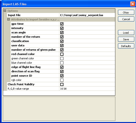
1. Select Modules | File | Shapes | Import | Import LAS Files.
   
   The Import LAS Files dialog box appears.
   
2. Click the Input file field. Click the browse [...] button and select and open a LiDAR LAS file .e.g. noisy_serpent.las.
   
3. In the Attributes to import besides x,y,z list, toggle on all the attributes you want to retain.
   
   
   
4. Click Okay.
   
   The LAS file is loaded as a PointCloud.
   

Assign the SRTM elevations to each LiDAR point

1. Select Modules | Shapes | Grid | Grid Values | Add Grid Values to Shapes.
   
   The Add Grid Values to Shapes dialog box appears.
   
2. In the Shapes field, choose the LiDAR point cloud layer e.g. 01. noisy_serpent.
   
3. In the Grids field, click the [...] button. Choose the reprojected SRTM grid layer e.g. 01.N39W084.
   
   
   
4. Click Okay.
   
   The SRTM elevation values are added as a new attribute to the LiDAR point cloud layer.
   

Create a valid elevation indicator attribute from the LiDAR point and the SRTM elevation values
This part is the key to the workflow. The Calculator is used to create a field that counts two tests: (1) if a point is above the bottom of the SRTM envelope and (2) if a point is below the top of the SRTM envelope. A count of 2 means the point is within the SRTM envelope. 

1. Select Modules | Shapes | Point Clouds | Tools | Point Cloud Attribute Calculator.
   
   The Point Cloud Attribute Calculator dialog box appears.
   
2. In the Point Cloud field, choose the LiDAR point cloud layer e.g. 01. noisy_serpent.
3. In the Result field, choose [create].
4. In the formula field, type in the following (without spaces):
   
   ifelse(gt(c,n-100),1,0)+ifelse(lt(c,n+100),1,0)
   
   Note: the point cloud attribute fields are in alphabetical order a, b, c....etc. c indicates the z attribute, n indicates the SRTM elevation field in this example and 100 is half the thickness of the envelope around the SRTM elevation.
   
   Note: the statement says that if the point z is greater than the bottom of the SRTM envelope (n-100) then assign 1, otherwise assign 0; and if the point z is less than the top of the envelope (n+100), then add another 1. Otherwise add 0.
   
5. In the Output Field Name field, type in valid.
6. In the Field data type field, change to 2 byte signed integer.
   
   
   
   
7. Click Okay.
   
   The Shapes point layer is created with a new attribute field valid containing values 1 and 2.
   

Filter out the LiDAR points outside the SRTM envelope

1. Select Module | Shapes | Points | Point Filter.
   
   The Points Filter dialog box appears.
   
2. In the Points field, choose the previously created point cloud layer e.g. 02. noisy_serpent_valid.
   
3. In the Attribute field, choose the field created previously e.g. valid.
   
4. In the Filtered Points field, choose [create].
   
5. In the Filter Criterion field, choose keep maxima (with tolerance). Leave the tolerance at 0.
   
   
   
   
6. Click Okay.
   
   The filtered Shapes point layer 01.noisy_serpent_valid[Filtered] is created. This layer contains only the LiDAR points inside the SRTM envelope.
   

Save as LAS

Before the filtered points can be saved as a LAS file, the Shapes point layer has to be converted to a point cloud layer. 

1. Select Module | Shapes | Point Cloud | Conversion | Point Cloud from Shapes.
   
   The Point Cloud from Shapes dialog box appears.
   
2. In the Shapes field, choose the Shapes point layer e.g. 01. noisy_serpent_valid[Filtered].
   
3. In the Z Value field, choose Z.
   
4. In the Output field, choose all attributes.
   
   
   
5. Click Okay.
   
   The Shapes point layer is converted to a point cloud layer 03. noisy_serpent_valid[Filtered].
   
   
6. Select Modules | File | Shapes | Export | Export LAS Files.
   
   The Export LAS Files dialog box appears.
   
7. In the Point Cloud field, choose the filtered point cloud layer e.g. 03. noisy_serpent_valid[Filtered].
   
8.  For each LAS field to export out, change the [not set] value to the appropriate attribute field.
   
9. If necessary, enter values in the Offset X, Offset Y fields that match the original LAS file.
   
10. Optional. Change the Point Data Record field accordingly e.g. to version 2.
    
11. In the Output field, define the output file name e.g. clean_serpent.las.
    
    
    
12. Click Okay.
    
    The filtered output LAS file is created without the zingers.
    

Detect changes between 2 polygon layers in gvSIG

gvSIG can be used to identify the spatial changes between two polygon vector layers. This can be done by using the Geoprocessing tools' Analysis Overlay difference function. An illustration of this is described below using the scenario of identifying the new vegetation growth and the loss of vegetation cover between a period of time.

Identify new vegetation growth

1. Start gvSIG OADE. Open a map view. Load and display two polygon layers e.g. vegetation2001.shp and vegetation2011.shp.
   
   
2. Select View | Geoprocessing tools.
   
   The Geoprocessing tools dialog appears.
   
3. Expand the nodes Geoprocessing tools | Analysis | Overlay. Select Difference. Click Open Tool.
   
   The Analysis tools dialog box appears.
   
4. In the Input layer field, choose vegetation2011.
5. In the Overlay layer field, choose vegetation2001.
6. In the Output layer field, type in the output file name, e.g. C:\temp\new_growth.shp.
7. Click OK.
   
   The polygons representing the new vegetation growth is created.
   

Identify the loss in vegetation cover

1. If the Geoprocessing tools dialog is not opened, then select View | Geoprocessing tools.
   
   The Geoprocessing tools dialog is displayed.
2. Expand the nodes Geoprocessing tools | Analysis | Overlay. Select Difference.
3. Click Open tool.
   
   The Analysis tools dialog box appears.
   
4. In the Input layer field, choose vegetation2001.
5. In the Overlay layer field, choose vegetation2011.
6. In the Output layer field, type in the output file name e.g. C:\temp\loss_of_vegetation.shp.
7. Click OK.
   
   The polygons representing the loss in vegetation cover are created.
   

Create geo-referenced heat maps Google Mapplet

Comma-separated-values (CSV) of statistical data in the format latitude, longitude, and magnitude can be imported and visualized as heat maps in Google Maps using this custom mapplet. An example screenshot is shown below.



While the heat maps feature is already possible using the Google Docs FusionTable object, the heat maps created from this Mapplet is done using the HTML5 canvas object via the Javascript heatmap.js library. On  top of that, the Mapplet provides the option to export out the heat map image file along with supporting geo-referenced information in the form of world and projection files.

To run the Mapplet, click this link http://dominoc925-pages.appspot.com/mapplets/vheatmap.html.

The Mapplet's sidebar contains a few button commands that should be obvious - Import, Export, Fit and Clear.

Clicking the Import button brings up the Import Points dialog. 

Copy and paste your comma-separated-values data into the text box. The data must be comma delimited and in  the following order: latitude, longitude, and magnitude. Alternatively, click Use random samples to let the Mapplet randomly create CSV data for demonstration purposes. 

Then click Start Import to create the heat map. 

Click  the Export button to export the heat map and supporting files. This will bring up the Export Heatmap dialog box. 

To save out the heat map image, right click on the image preview and choose Save image as. 

Next, click on the World file text box and press +C to copy the contents to the clipboard. Then paste inside a text editor and save the world file with the same file name but with the prefix *.pgw. 

Similarly, click on the Projection text box and press +C. Then paste in a text editor and save the contents into a projection file with the same file name prefix but with the extension *.prj. 

Once the image, world file and projection have been exported, the heat map can be displayed and overlaid with other geo-spatial data in any GIS software e.g. Global Mapper as shown below.