Using Saga GIS' Terrain Analysis Swath Profile (interactive) function

Saga GIS has a couple of interactive terrain profiling functions, a single profile and a swath profile. This post shows how to use the interactive swath terrain profile command.

Load a grid file such as a USGS SRTM file

1. Run Saga GIS. Select Geoprocessing | File | Grid | Import | Import USGS SRTM Grid.
   
   The Import USGS SRTM Grid dialog box appears.
   
2. Click the Browse button in the Files field. Choose an SRTM file e.g. N21E093.hgt.
   
   
3. Click Open.
   
   
4. Click Okay.
   
   The SRTM file is loaded and shown in the Data tab.
   

Start the swath profile command

1.  Under the Data tab, mouse right click on the loaded grid file e.g. N21E093.
2. In the pop up context menu, choose Add to Map.
   
   The grid file is displayed in a map window.
   
3. Select Geoprocessing | Terrain Analysis | Profiles | Swath Profle [Interactive].
   
   The Swath Profile dialog box appears.
   
4. In the Grid system field, choose the loaded grid file's system e.g. 0.000833; 1201x 1201y; 93x 21y option.
5. In the DEM field, choose the loaded grid file, e.g. N21E093.
6. Optional. Change the Swath Width if necessary.
   
   The message Interactive tool execution has been started is displayed in the Messages pane.

Digitize the swath profile

1. In the Toolbar, click the Action icon (that looks like a black NW arrow).
2. In the map window, click a few points to draw the swath profile.
   
   
   
3. To complete the drawing, press the mouse right button.
4. To exit the interactive command, select Geoprocessing | Swath Profle [Interactive].
   
   The Tool Execution prompt appears.
   
5. Click Yes.
   
   The message: "Interactive tool execution has been stopped" is shown in the Messages pane.
   
   Note: This may take a while as the command will sample the terrain to calculate the points.

Display the swath profile graphically

1.  In the Data pane, mouse right click on the newly created profile points e.g. Profile [N21E093].
   
   
2. In the pop up menu, choose Attributes | Diagram.
   
   The Properties dialog box appear.
   
3. In the X Axis Values field, choose D (for Distance).
4. In the X Axis Label field, choose D.
5. In the Attributes field, toggle on Z, Z [min], Z[max].
6. Set other options if necessary.
7. Click Okay.
   
   The profile line(s) are displayed.
   

Use Saga GIS to create Voronoi or Thiessen polygons

The new version of Saga GIS 2.1 has a functional Thiessen polygon command. Previously, a bug in the function creates erroneous polygons. Here is an example of using the command to create Voronoi or Thiessen polygons from discrete points with some polygon clipping thrown in for aesthetic effects. The example shows how to create polygons of cities in the great State of Texas.

1. Start SAGA GIS. Load and display the cities and the state boundary polygon in a map view.
   
   
   
2. Select Modules | Shapes | Points | Thiessen Polygons.
   
   The Thiessen Polygons dialog box appears.
   
   
3. In the input Points field, choose the point layer, e.g. 01. cities_in_texas.
   
4. In the output Polygons field, select create. Click Okay.
   
   The Thiessen polygons layer (02. cities_in_texas [Thiessen Polygons] is created. The polygons are spread out over some arbitrary four points.
   
   
5. Select Modules | Shapes | Polygons | Polygon Clipping.
   
   The Polygon Clipping dialog box appears.
   
   
6. In the Clip Features field, select the State boundary polygon layer, e.g. 01. texas.
   
7. Select the Input Features field and click the [...] button.
   
   The Input Features dialog box appears.
   
   
8. In the left list, select the Thiessen Polygons layer, e.g. 02. cities_in_texas [Thiessen Polygons]. Click the > button. Click Okay.
   
   The Input Features dialog box is closed.
   
9. Click the Okay button.
   
   The Thiessen polygons are nicely clipped to the State polygon.
   

Remove noisy spikes from LiDAR data using SAGA GIS and SRTM data

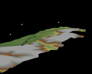
LiDAR data collected from the field contains noise in the form of spikes or zingers (extremely high or low points) and/or clouds. Typically these erroneous points are reclassified as noise from the point cloud by using high-low filters, median filters or other statistical methods. An example is shown in the screenshot below.


I have in mind using the globally available Shuttle Radar Topography Mission (SRTM) data to form an envelope to filter away the extreme noise points using SAGA GIS. SRTM data can be downloaded from http://www2.jpl.nasa.gov/srtm/.

From the SRTM elevation data, a height value can be added and subtracted to form a volume envelope. Any LiDAR points inside the envelope are valid points while any points outside the envelope are noise. The following illustrates a possible workflow.

Load and reproject an SRTM tile to match the LiDAR data

1. Start SAGA GIS.
2. Select Modules | File | Grid | Import | Import USGS SRTM Grid.
   
   The Import USGS SRTM Grid dialog appears.
   
   
3. Click the Files field. Then click the browse [...] button. Browse and select an SRTM file e.g. N39W084.hgt. Click Open. Click Okay.
   
   The SRTM data is loaded.
   
   Note: the SRTM data is in a geographical latitude-longitude coordinate system while the LiDAR data is in a projected coordinate system e.g. UTM 17 North.
   
4. Select Modules | Projection | Coordinate Transformation (Grid).
   
   The Coordinate Transformation (Grid) dialog box appears.
   
   
5. In the EPSG Code | Projected Coordinate Systems field, choose a coordinate system e.g. WGS 84 / UTM zone 17N.
6. In the Data Objects | Grid system field, choose the SRTM grid system e.g. 0.000833; 1201x 1201y; -84x 39y.
7. In the Data Objects | Grid system | source field, choose the SRTM grid layer e.g. 01.N39W084.
   
   
   
8. Click Okay.
   
   The User Defined Grid dialog box appears.
   
   
   
9. Click Okay.
   
   The SRTM grid is reprojected into UTM 17 North.
   
   Note: there are now two SRTM grid layers with the same name. For clarity, we shall remove the first SRTM grid layer.
   
10. In the Data tab of the Workspace pane, select the first SRTM grid layer e.g. 01. N39W084.
    
11. Press the mouse right click button. In the pop up menu, select Close.
    
    
    
12. Click Yes and Okay.
    
    The original SRTM grid layer is removed.

Load the LiDAR LAS file

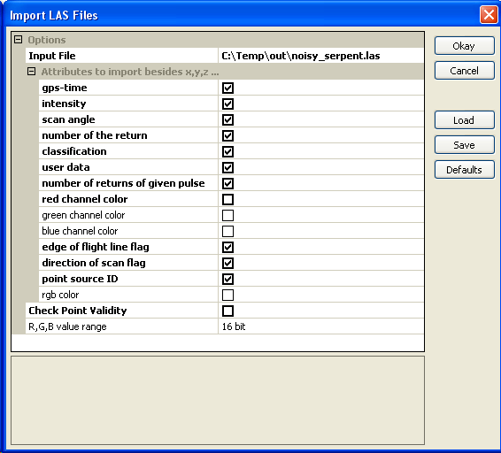
1. Select Modules | File | Shapes | Import | Import LAS Files.
   
   The Import LAS Files dialog box appears.
   
2. Click the Input file field. Click the browse [...] button and select and open a LiDAR LAS file .e.g. noisy_serpent.las.
   
3. In the Attributes to import besides x,y,z list, toggle on all the attributes you want to retain.
   
   
   
4. Click Okay.
   
   The LAS file is loaded as a PointCloud.
   

Assign the SRTM elevations to each LiDAR point

1. Select Modules | Shapes | Grid | Grid Values | Add Grid Values to Shapes.
   
   The Add Grid Values to Shapes dialog box appears.
   
2. In the Shapes field, choose the LiDAR point cloud layer e.g. 01. noisy_serpent.
   
3. In the Grids field, click the [...] button. Choose the reprojected SRTM grid layer e.g. 01.N39W084.
   
   
   
4. Click Okay.
   
   The SRTM elevation values are added as a new attribute to the LiDAR point cloud layer.
   

Create a valid elevation indicator attribute from the LiDAR point and the SRTM elevation values
This part is the key to the workflow. The Calculator is used to create a field that counts two tests: (1) if a point is above the bottom of the SRTM envelope and (2) if a point is below the top of the SRTM envelope. A count of 2 means the point is within the SRTM envelope. 

1. Select Modules | Shapes | Point Clouds | Tools | Point Cloud Attribute Calculator.
   
   The Point Cloud Attribute Calculator dialog box appears.
   
2. In the Point Cloud field, choose the LiDAR point cloud layer e.g. 01. noisy_serpent.
3. In the Result field, choose [create].
4. In the formula field, type in the following (without spaces):
   
   ifelse(gt(c,n-100),1,0)+ifelse(lt(c,n+100),1,0)
   
   Note: the point cloud attribute fields are in alphabetical order a, b, c....etc. c indicates the z attribute, n indicates the SRTM elevation field in this example and 100 is half the thickness of the envelope around the SRTM elevation.
   
   Note: the statement says that if the point z is greater than the bottom of the SRTM envelope (n-100) then assign 1, otherwise assign 0; and if the point z is less than the top of the envelope (n+100), then add another 1. Otherwise add 0.
   
5. In the Output Field Name field, type in valid.
6. In the Field data type field, change to 2 byte signed integer.
   
   
   
   
7. Click Okay.
   
   The Shapes point layer is created with a new attribute field valid containing values 1 and 2.
   

Filter out the LiDAR points outside the SRTM envelope

1. Select Module | Shapes | Points | Point Filter.
   
   The Points Filter dialog box appears.
   
2. In the Points field, choose the previously created point cloud layer e.g. 02. noisy_serpent_valid.
   
3. In the Attribute field, choose the field created previously e.g. valid.
   
4. In the Filtered Points field, choose [create].
   
5. In the Filter Criterion field, choose keep maxima (with tolerance). Leave the tolerance at 0.
   
   
   
   
6. Click Okay.
   
   The filtered Shapes point layer 01.noisy_serpent_valid[Filtered] is created. This layer contains only the LiDAR points inside the SRTM envelope.
   

Save as LAS

Before the filtered points can be saved as a LAS file, the Shapes point layer has to be converted to a point cloud layer. 

1. Select Module | Shapes | Point Cloud | Conversion | Point Cloud from Shapes.
   
   The Point Cloud from Shapes dialog box appears.
   
2. In the Shapes field, choose the Shapes point layer e.g. 01. noisy_serpent_valid[Filtered].
   
3. In the Z Value field, choose Z.
   
4. In the Output field, choose all attributes.
   
   
   
5. Click Okay.
   
   The Shapes point layer is converted to a point cloud layer 03. noisy_serpent_valid[Filtered].
   
   
6. Select Modules | File | Shapes | Export | Export LAS Files.
   
   The Export LAS Files dialog box appears.
   
7. In the Point Cloud field, choose the filtered point cloud layer e.g. 03. noisy_serpent_valid[Filtered].
   
8.  For each LAS field to export out, change the [not set] value to the appropriate attribute field.
   
9. If necessary, enter values in the Offset X, Offset Y fields that match the original LAS file.
   
10. Optional. Change the Point Data Record field accordingly e.g. to version 2.
    
11. In the Output field, define the output file name e.g. clean_serpent.las.
    
    
    
12. Click Okay.
    
    The filtered output LAS file is created without the zingers.
    

Counting trees using segmentation and vectorization in SAGA Gis

Digital surface models (DSM) and digital terrain models (DTM) derived from LiDAR datasets can be used to count the number of trees in an area. There are many methods available, some more complex than others. Here is another example of doing a simple tree count using SAGA GIS' Watershed Segmentation algorithm followed by the Vectorization function. The general steps are:

1. Load in the DSM and DTM grid datasets
2. Calculate the canopy heights
3. Smooth the canopy heights grid
4. Segment the canopy heights
5. Remove low canopy heights
6. Convert the segments to vector polygons

Load the DSM and DTM grid datasets

1. Start SAGA GIS. Load the DSM ArcGrid file e.g. C:\data\dsm.asc.
2. Load the DTM ArcGrid file e.g. C:\data\dtm.asc.

Calculate the canopy heights

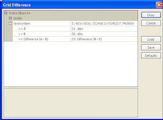
1. Select Modules | Grid | Calculus | Grid Difference.
   
   The Grid Difference dialog box appears.
   
2. In the Grid system field, choose the system of the source datasets, e.g. 683x 683y; 312480x 51952717y.
3. In the A field, choose the digital surface model grid, e.g. dsm.
4. In the B field, choose the digital terrain model grid, e.g. dtm.
5. Click Okay.
   
   The canopy height grid is created.
   

Smooth the canopy heights

1. Select Modules | Grid | Filter | Gaussian Filter.
   
   The Gaussian Filter dialog box appears.
   
2. In the Grid system field, choose the system of the source grid e.g. 683x 683y; 312480x 51952717y.
3. In the Grid field, choose the canopy height grid, e.g. Difference (A-B).
4. In the output Filtered Grid field, choose Create.
5. In the Search Radius field, choose a value to approximate the tree radius e .g. 5.
6. Click Okay.
   
   The smoothed canopy height grid is created.
   

Segment the smoothed canopy heights

1. Select Modules | Imagery | Segmentation | Watershed Segmentation.
   
   The Watershed Segmentation dialog box appears.
   
2. In the Grid system field, choose the grid system of the smoothed grid layer.
3. In the source Grid field, choose the smoothed grid layer e.g. Difference (A-B) [Gaussian Filter].
4. In the Output field, choose Seed.
5. Make sure the Method is set to Maxima.
6. Click Okay.
   
   The canopy heights grid layer is segmented according to maximum heights.
   

Apply a height break limit (removing segments below a certain height)

1. Select Modules | Grid | Calculus | Grid Calculator.
   
   The Grid Calculator dialog box appears.
   
2. In the Grid system field, choose the system of the segmented layer.
3. In the Grids field, click the browse button. In the Grids dialog box that pops up, double click on the segmented  grid layer e.g. "Difference (A-B) [Gaussian Filter][Segments]". Click Okay.
4. In the Formula field, type in the following: ifelse(lt(a,5),-99999,a).
   
   Note: if the grid value is less than 5, then change the grid value to voids (-99999).
5. Click Okay.
   
   The grid layer with no values below the height break limit is created.
   

Convert the segments into vectors

1. Select Modules | Shapes | Grid | Vectorization | Vectorising Grid Classes.
   
   The Vectorising Grid Classed dialog box appears.
   
2. In the Grid system field, choose the system of the previously created grid layer.
3. In the Grid field, choose the grid layer created in the previous step e.g. "Calculation [ifelse(lt(a,5),-99999,a)]".
   
   
   
   
4. Click Okay.
   
   The vector polygon layer is created.
5. Select the shape polygon layer in the Data tab. Then click the Description tab.
   
   The number of shapes shows the approximate count of the number of trees above a height break limit.
   
   
   
   
   The polygons can be displayed as table attribute records as shown below.