Take Geospatial files on the go with the Shapefiler App

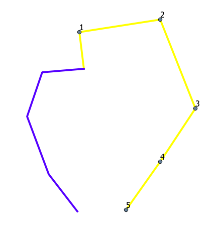
 Easily load and visualize multiple GeoJSON and Shapefiles with this powerful mapping tool. The app automatically assigns overlay colors, but you have full control over the styling—customize icons, colors, and opacity through the layer properties menu. Tap on polygons, lines, and markers to view detailed feature attributes. Quickly find specific locations with the built-in free text search, making navigation effortless. Whether you're a GIS professional or a mapping enthusiast, this app provides an intuitive way to explore spatial data on your device. 

Key features

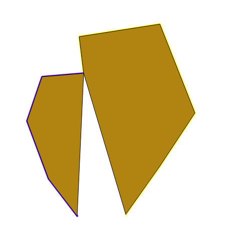
Load multiple Geospatial files: Overlay GeoJSON and Shapefiles over a choice of base map tiles.

Integrated tabular and map views: Tap on a data table record to locate the corresponding feature on the map

Multiple coordinate reference systems: Source Geospatial GeoJSON and Shapefiles in various coordinate reference systems can be reprojected to the standard World Mercator projection for display.

Free text search: Easily search features by text and locate on the map. 

For more detailed information, visit https://dominoc925.blogspot.com/p/shapefiler-help.html. 

Download and try out the Shapefiler app from the following stores:

Example efficient two pass Spatialite query to find if a point is inside a polygon

A spatial query can be expensive to run in terms of CPU processing power. In order to improve the query performance, typically, a first pass query is done to reduce the candidates first before running a second pass query to do actual spatial query. The following is an example using SpatiaLite to perform a two pass spatial query to find whether a point is contained within a polygon.

Point 1 is totally outside of any polygons; Point 2 is outside but within a bounding rectangle of a polygon; Point 3 is totally inside a polygon.

The two pass SpatiaLite query has the following syntax.
Note: the first approximate query uses the MBRCONTAINS function and the second finer query uses the ST_CONTAINS function.

SELECT ST_CONTAINS(polygonGeometry, geomfromtext('POINT(116.4688 -31.5502)', 4326))
FROM(
SELECT
polygonGeometry,
MBRCONTAINS(polygonGeometry, geomfromtext('POINT(116.4688 -31.5502)', 4326)) AS inMBR
FROM
(
SELECT geometry AS polygonGeometry FROM MyPolygon
)
WHERE inMBR = 1
)

Case 1: Totally outside 
For Point 1 (Totally outside), the query returns no rows since the point is outside of any bounding rectangles, as shown in the screenshot below.


Case 2: Outside of any polygons but within a bounding rectangle
For Point2, the query returns a result of 0 value, since the point is inside a bounding rectangle but outside of any polygon.

Case 3: Totally inside a polygon
For Point 3, the query returns a result of 1 since the point is inside a bounding rectangle and also inside a polygon.

Using SpatiaLite GUI to create a point geometry table from an ordinary table

Sometimes I have an ordinary table with numerical latitude and longitude columns and I need to construct a point geometry table from the records in the normal table, e.g. stations_raw. An example of such a table is shown in the screenshot below.

In the SpatiaLite GUI, enter the following SQL command to create a new table named stations:
CREATE TABLE stations AS 
SELECT
PK_UID,
code,
name,
ST_GeomFromText(
'POINT('||lng||' '||lat||')', 
4326
)
AS Geometry
FROM stations_raw

Note: 4326 in the example command is just the geographical coordinate system SRID of the data.

Execute the command.


The table stations is created.


The table is still a non-spatial table. In order to change it to a spatial table, the following steps need to be done.

1. In the SpatiaLite GUI, press mouse right click on the geometry column.
   
   
   
2. In the pop up menu, choose Recover geometry column,
   
   The Recover Geometry column dialog box appears.
   
   
3. In the SRID field, type in the data's SRID e.g. 4326 for geographical latitude and longitude data.
   
4. In the Dims field, choose the appropriate dimensions of the data, e.g. XY for 2-D.
   
5. In the Geometry field, choose the appropriate geometry of the data, e.g. POINT for point data.
   
6. Press OK.
   
   If the parameters are correct, the following message will appear.
   
   
   The GUI should show the table as a spatial table (with a globe).
   

Example SpatiaLite query to find neighbors of a polygon

A common spatial query is to find all the neighbor polygons touching a subject polygon. The screenshot below shows a SpatiaLite database of selected country feature polygons.

If you want to find all the neighboring countries of the country Canada, the following SpatiaLite SQL query can be used.
select b.name
from country a, country b
where touches(a.geometry, b.geometry)
and a.name = 'Canada'


The result 'USA' is returned.
 

Join 2 lines in QGIS

There is a useful plugin in QGIS - Join Lines, that can be used to join two lines into one; reversing the direction of vertices of one line if necessary. This can be useful if you want to construct polygons later on from the lines. The following example shows a problem that can arise if generating polygons from lines that have opposing directions.

The screenshot below shows the counter-clockwise digitized direction of a line feature.


The other line feature is digitized in a clockwise direction.


If a polygon is constructed using the QGIS Line to Polygon function, the following polygon will be generated.


Using the Join Lines command

1. If the Join Lines plug-in is not installed, select Plug-ins | Manage and install plug-ins and install the Join Lines plug-in.
   
   
   
2. In the map view, select two lines.
   
   
   
3. Select Vector | Join two lines | Join two lines.
   
   
   
4. Select Layer | Toggle editing.
   
   
   
5. Click Save.
   
   The joined line is saved.
   

If the joined lines are used to generate a polygon, the following area geometry will be constructed.

Merge SpatiaLite polygon geometries with the GUnion operator in QGIS

I wanted to merge two polygon geometries in a SpatiaLite database (an example is the land feature layer shown in the screenshot below) into a single geometry using QGIS.

Two SpatiaLite polygons labelled with the primary key id number.

In QGIS, the usual command to perform this task is the Union command, but unfortunately it creates only Shapefiles. The alternative is to use the QSpatiaLite plug-in and run some SQL commands to do the job. The following steps show how to merge two polygons into one polygon using the SpatiaLite GUnion operator.

1. In QGIS, select Database | SpatiaLite | QSpatiaLite.
   
   The QSpatiaLite dialog box appears.
   
2. Note down the primary key numbers or any suitable identifier of the polygons to be merged, e.g. pkuid 10 and 20.
3. In the SQL tab field, type in the SQL command.
   
   SELECT GUNION
   (
   (SELECT geometry FROM land WHERE pkuid = 10)
   ,
   (SELECT geometry FROM land WHERE pkuid = 20)
   )
   AS geometry
   
   
4. Click Run SQL.
   
   A temporary new geometry object is created.
   
   
   Note: if the above SQL command execution is successful, then it is fine to proceed to create a new merged polygon feature and delete the original two polygons.
5. In the SQL tab, type in the following SQL command to create and insert a merged polygon feature record.
   
   INSERT INTO land (geometry)
   SELECT GUNION
   (
   (SELECT geometry FROM land WHERE pkuid = 10)
   ,
   (SELECT geometry FROM land WHERE pkuid = 20)
   )
   AS geometry
   
6.  Click Run SQL.
   
   A new row is inserted into the land table.
   
7. In the SQL tab, type in the SQL command to delete the original two polygon features.
   
   DELETE FROM land WHERE pkuid = 10 OR pkuid = 20
   
   
8. Click Run SQL.
   
   The original polygon features are deleted.
9. Refresh the map view by toggling the land feature display off and on.
   
   The merged polygon is displayed.
   

Identifying digital elevation model files with erroneous elevations in batch

A DEM file

Recently I had to identify ESRI ArcGrid ASCII files of digital elevation models with very low elevation values (below zero). If I had one or two files, then I could easily open up the file in Global Mapper or Saga GIS. But there were several hundred DEMs, which made that impractical. Luckily the free open source software GDAL has a utility gdalinfo that can generate statistics about a DEM in batch. The following example shows how to use gdalinfo to look for extreme low (or high) spikes in elevation.

1. Open up a Windows Command Prompt.
   
2. Type in the following:
   
   C:> gdalinfo -stats inputDEM.asc > output.txt
   
   Note: to append to an output file, use double ">" as below.
   
   C:> gdalinfo -stats inputDEM.asc >> output.txt
   
   
   
   Note II: For hundreds of files, simply put these commands into a batch script.
3. Open up the output file e.g. output.txt in a text editor. Find the statistical values - minimum, maximum that are above or below the valid elevation ranges to identify the DEM files with erroneous values.
   
   

Free 30 day trial LiDAR LAS Viewer from GeoKno

I tried out a free 30 day trial software LASViewer from GeoKno on some of my LiDAR LAS files. I found the software to have good display point cloud rendering functions, and decent windowing and navigation functions. The point cloud analysis and measurement functions are okay except for the lack in cross section profiling functions. However, I found the software to perform poorly in terms of speed and stability on mid size and larger LAS files.


Displaying a LAS file

1. To open and display a LAS file, just drag and drop the file onto the LASViewer application.
   
   The Open Dialog pops up.
   
2. Optional. In the Point skip option field, type in the number of points to decimate e.g. 10, if you want to reduce the number of points to display.
3. Click OK.
   
   The point cloud is displayed.
   
   
   Note: LASViewer does not seem to be able to display more than one LAS file in the same view

Point cloud rendering

The point cloud can be displayed in a variety of ways including by color ranges (earth tones or blue to red), intensity gray scale, flight source id, classification, RGB. The software has the capability to render the cloud as discrete points, or as a surface wire frame or shaded triangles, as shown in the screenshot below.
 

Overlaying with vector Shapefiles
I found it quite useful to be able to overlay a vector ESRI Shapefile with the LiDAR point cloud. A common task is to examine the point cloud with the area of interest (AOI) vector polygon. To reference a Shapefile, simply do the following:

1. Click Display | Display with SHP.
   
   The Open Dialog appears.
   
2. Browse and select a Shapefile, e.g. contour.shp. Click Open.
   
   The Shapefile is overlaid over the point cloud.
   

Examine point information
Another typical task is to examine information about a LiDAR point to review the return value or classification value or to determine the elevation. LASViewer has the Point Information Tool that can be used to display the LiDAR point values in a separate window, as shown below.

1. Click Tools | Point.
2. Click on a LiDAR point.
   
   The Point Information is displayed. 

Measure geodesic area on Google Maps

This Google Mapplet can be used to measure polygonal area and perimeter on a sphere in Google Maps using an open source library GeographicLib. Using the mapplet is easy - simply place click three or more points on the Google Maps backdrop to define a polygon; the area and perimeter values will be displayed in the centroid of the polygon.



The default units of measurement for area and perimeter, as well as the polygon boundary color can be changed by selecting the desired values in the right pane.

Once the measurement polygon has been placed on the map backdrop, the vertices can be adjusted either by manually dragging a vertex marker with the mouse or by clicking the vertex marker and entering refined latitude and longitude values.

A vertex marker can be deleted by clicking on the vertex marker and selecting the Delete option.

The mapplet can be found at this link http://dominoc925-pages.appspot.com/mapplets/geoarea.html.