Convert Geoids from BYN to GTX format with this WebApp

This WebApp came about because I wanted to use some Geoid files for some vertical datum corrections with Proj (which uses .gtx format) but could only find Geoid files in Natural Resources Canada's .byn format.

1. To convert Geoid BYN files to GTX, open up a browser to the following url: https://dominoc925-pages.appspot.com/webapp/byn2gtx/index.html.
   
   
   The WebApp is loaded.
   
   
   
   
   
   
   
   
   
    
2. Click the Add File button.
   
   The File Upload dialog appears.
   
   
   
   
   
3. Browse and select a .byn file e.g. EGM96.byn. Click Open.
   
   
   The Geoid file is displayed in a list and the Convert button is enabled.
   
   
   Note: the Geoid .byn is loaded locally to the browser and not transferred to some server on the Internet.
   
   
   
   
4. Click the Convert button.
   
   The Geoid file is converted into .gtx format and the Process log and Save As icons are enabled.
   
   
   
   
   
   
5. Optional. To view the process log, click the Show Process Log icon.
   
   The process log messages are displayed.
   
   
   
   
   
   
6. To save the converted .gtx Geoid locally, click the Save Converted File icon.
   
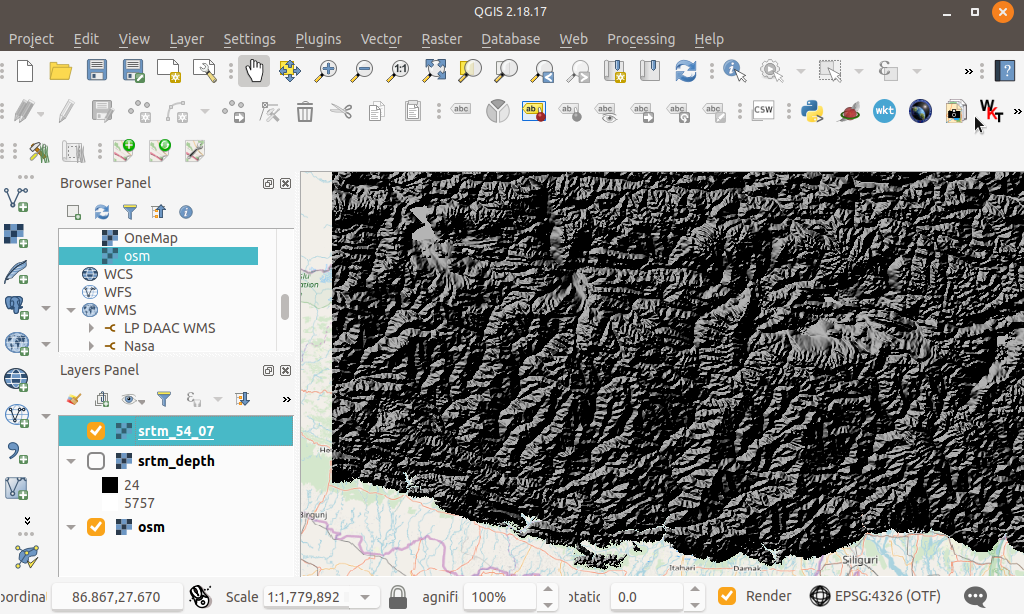
   The Geoid file is saved.
   
   
   
7. Optional. If necessary, you can use a GIS software like QGIS to display the converted .gtx file, as shown below.
   
   
    
   
    

Using Saga GIS' Terrain Analysis Swath Profile (interactive) function

Saga GIS has a couple of interactive terrain profiling functions, a single profile and a swath profile. This post shows how to use the interactive swath terrain profile command.

Load a grid file such as a USGS SRTM file

1. Run Saga GIS. Select Geoprocessing | File | Grid | Import | Import USGS SRTM Grid.
   
   The Import USGS SRTM Grid dialog box appears.
   
2. Click the Browse button in the Files field. Choose an SRTM file e.g. N21E093.hgt.
   
   
3. Click Open.
   
   
4. Click Okay.
   
   The SRTM file is loaded and shown in the Data tab.
   

Start the swath profile command

1.  Under the Data tab, mouse right click on the loaded grid file e.g. N21E093.
2. In the pop up context menu, choose Add to Map.
   
   The grid file is displayed in a map window.
   
3. Select Geoprocessing | Terrain Analysis | Profiles | Swath Profle [Interactive].
   
   The Swath Profile dialog box appears.
   
4. In the Grid system field, choose the loaded grid file's system e.g. 0.000833; 1201x 1201y; 93x 21y option.
5. In the DEM field, choose the loaded grid file, e.g. N21E093.
6. Optional. Change the Swath Width if necessary.
   
   The message Interactive tool execution has been started is displayed in the Messages pane.

Digitize the swath profile

1. In the Toolbar, click the Action icon (that looks like a black NW arrow).
2. In the map window, click a few points to draw the swath profile.
   
   
   
3. To complete the drawing, press the mouse right button.
4. To exit the interactive command, select Geoprocessing | Swath Profle [Interactive].
   
   The Tool Execution prompt appears.
   
5. Click Yes.
   
   The message: "Interactive tool execution has been stopped" is shown in the Messages pane.
   
   Note: This may take a while as the command will sample the terrain to calculate the points.

Display the swath profile graphically

1.  In the Data pane, mouse right click on the newly created profile points e.g. Profile [N21E093].
   
   
2. In the pop up menu, choose Attributes | Diagram.
   
   The Properties dialog box appear.
   
3. In the X Axis Values field, choose D (for Distance).
4. In the X Axis Label field, choose D.
5. In the Attributes field, toggle on Z, Z [min], Z[max].
6. Set other options if necessary.
7. Click Okay.
   
   The profile line(s) are displayed.
   

Create a Facebook 3D Photo of a digital elevation model using QGIS

Facebook has a 3D photo feature which brings perspective and movement to the Facebook news feed and timeline images. A live example can be seen embedded here:


Normally these images are created using RGB-D cameras, where D stands for depth. However it is also possible to workaround it without a RGB-D camera by uploading to Facebook two images - an RGB image and its corresponding grayscale depth image, and making sure the depth image has the same name as the RGB image with a '_depth' suffix. The depth image is grayscale only with values ranging from dark to light -  the dark pixels representing the furthest pixels and the light pixels representing the nearest pixels.

Using the ideas above, the following steps illustrate how to create a Facebook 3D Photo image from a SRTM digital elevation model (DEM) using QGIS.

1. Startup QGIS. Create a new project. If the canvas background is not already black, select Project | Project Properties.
   
   The Project Properties dialog box appears.
   
2. In the Background color field, change the color to black. Click OK.
   
   The canvas background becomes black.
   
3. Drag and drop a DEM file onto the canvas e.g. srtm_54_07.tif.
   
    
4.  Optional. To serve the purpose of having a background, an OpenStreetMap (OSM) layer is displayed behind the DEM layer.
   
   
5. Optional. To display only DEM heights above an elevation of interest, e.g. 200 meters, right click on the DEM layer and choose Properties. Then add in a new transparent entry to the transparent pixel list from 0 to 200 meters, as shown below. Then click OK.
   
   The Layer Properties dialog box appears.
   
   
   
   The DEM display is updated.
   
   
6. Make a duplicate of the DEM layer by right clicking on the DEM layer and choosing Duplicate. Rename the copy as 'depth' as it will serve to generate a depth image later on.
   
   
7. Right click on the top most DEM layer and choose Properties. In the Layer properties dialog box, click Style.
   
   
8. Change the Render Type to Hillshade. Click OK.
   
   The DEM layer is now rendered as a hill shade.
   
9. Make a duplicate copy of the hill shaded DEM layer by right clicking the layer and choosing Duplicate. Rename the copy as 'hillshade' as shown below.
   
   
10. Right click on the top most DEM layer and choose Properties. Select the Style tab.
    
    
11. In the Rendering type field, choose Singleband pseudocolor. Choose a suitable color gradient e.g. Spectral and toggle Invert if necessary. Choose a suitable Blending mode e.g. Screen.
    
    
12. Click OK.
    
    The DEM layer is rendered with a colored gradient.
    
13. With the gradient colored, hill shaded and OSM layers displayed on and the depth layer displayed off, export out the canvas by selecting Project | Save as image and specifying an output file name e.g. srtm.png.
    
    The srtm image is generated.
    
14. Now turn off the gradient, hill shaded and OSM layers. Turn on the depth layer as shown below.
    
    
    
    
    Select Project | Save as image to export out the depth image with a '_depth' suffix e.g. srtm_depth.png.
    
    The srtm_depth image is generated.
    
15. Now open up Facebook in a browser and click the Post Photo/Video button.
    
    The File Upload dialog box appears.
    
16. Browse and select the generated srtm.png and srtm_depth.png files. Click Open.
    
    Facebook generates the 3D Photo.
    
    
    A live example is available here at https://www.facebook.com/permalink.php?story_fbid=1251984134967474&id=101193703379862

Use PDAL to generate a DEM from a LiDAR LAS file

PDAL can be used to generate a GeoTIFF digital elevation model (DEM) from a LiDAR point cloud LAS file via the GDAL writer driver. The resultant elevation GeoTIFF file may not be displayed as what is expected in some software such as Global Mapper because the PDAL generated file can have one or more bands of data including an alpha channel, depending on the PDAL options used; refer to https://www.pdal.io/stages/writers.gdal.html for the types of output bands that can be written to the DEM GeoTIFF file. For normal display, it might be necessary to separate the bands into individual files - in this post, the OTB (Orfeo Tool Box) otbcli_splitImage executable is used.

The following steps show how to generate a GeoTIFF DEM and split the resultant file into separate bands.

Generate the DEM

1. Open up a text editor. Type in the following JSON text. Save the text into a file e.g. pdal_dtm.json
   
   
   
   Note: the JSON pipeline text will do the following:
   (a) Load in a LAS file e.g. autzen.laz
   (b) Filter away non-ground classified point
   (c) Write only the mean Z values to a GeoTIFF file dem.tif with a resolution of 10 meters
   
2. Open up the OSGeo4W Command Prompt.
   
   The Command Prompt appears.
   
3. Type in the PDAL command to process the pipeline. Run the command.
   
   C:\> pdal pipeline pdal_dtm.json
   
   The GeoTIFF file dem.tif is generated.
   

Splitting the bands

Displaying the resultant dem.tif containing only the mean Z band in QGIS will show something resembling a grayscale terrain with masked areas, as shown in the screenshot below.

However, displaying the resultant GeoTIFF in Global Mapper will show a black rectangle, as shown below, due to the presence of an alpha channel. This need to be removed for proper interpretation of the elevation data.

To split the bands, do the following:

1. In the OSGeo4W Command Window, type in the command:
   
   C:\> otbcli_splitimage -in dem.tif -out split.tif
   
   
   
   The input file dem.tif is split into separate files with a numbered suffix starting from 0 e.g. split_0.tif.
   
2. Now, the file can be displayed properly in Global Mapper.
   

Simple LiDAR ground points classification and segmentation using PDAL

PDAL (Point Data Abstraction Library) comes with a couple of options to segment point clouds by classifying LiDAR ground points (an example unclassified point cloud is shown below) - Simple Morphological Filter (SMRF) or Progressive Morphological Filter (PMF).

I have found the SMRF method to be fast and produce reasonable results while the PMF method seems to take a much longer time to do the job. The steps to run ground classification on a LAS file are describe below.

1. In Windows, open up the OSGeo4W Shell.
   
   The OSGeo4W Shell is displayed.
2. In the OSGeo4W prompt, type in and run the command:
   
   C:\> pdal translate -i unclassified.las -o ground.las smrf -v 4
   
   Notes:
   -i unclassified.las is the input file
   -o ground.las specifies the output file
   smrf is the option to apply the Simple Morphological Filter
   -v 4 is the processing messages verbosity level
   
   Processing messages appear.
   
3. Display the ground classified LAS file in a viewer.
   
   
   
   
4. To use the Progressive Morphological Filter to perform the ground classification, type in the following command:
   
   C:\> pdal translate -i unclassified.las -o ground.las pmf -v 4
   
   Notes:
   -i unclassified.las is the input file
   -o ground.las specifies the output file
   pmf is the option to apply the Progressive Morphological Filter
   -v 4 is the processing messages verbosity level

Normalize a Lidar LAS file with Fusion ClipData

There are occasions when it is necessary to normalise a LiDAR las point cloud file, i.e. removing the terrain heights. This can be useful if you are interested in the heights of objects e.g. vegetation canopy above the ground and not the undulations of the terrain below. An example of a las file point cloud is shown below; the shape of the terrain is very much evident.


The ClipData utility from the open source Fusion software can be used to normalise a LiDAR point cloud. The following steps illustrate how to normalise a point cloud.

1. In a Command Prompt, type in the following to convert a digital terrain model DTM from ESRI Ascii ArcGrid to Fusion's DTM format, using the ASCII2DTM.exe utility.
   
   C:\> ascii2dtm.exe output.dtm m m 0 0 0 0 input_dem.asc
   
   An example run is shown below.
   
   
2. At the prompt, type in the following.
   
   C:\> clipdata.exe /height /dtm:dakota_dem.dtm dakota.las output.las 606034 4889354 607400 4890580
   
   Note:
   /height tells the utility to normalise the point cloud
   /dtm:dakota_dem.dtm specifies the input digital terrain in Fusion's DTM format.
   dakota.las is the input las file
   606034 is the minimum bounding x value
   4889354 is the minimum bounding y value
   607400 is the maximum bounding x value
   4890580 is the maximum bounding y value
   
   An example run is shown below:
   
   
   A screenshot showing the normalised point cloud. Notice the point cloud no longer undulates with the terrain.