Segment individual trees from TLS point clouds with 3DForest

Identifying individual trees from point clouds scanned using Terrestrial LiDAR System (TLS can be easily segmented using this freely downloable software 3DForest. For more information about 3DForest, visit http://www.3dforest.eu/.

Note: although 3DForest has its own ground classification filter, I found it better to perform the ground / non-ground classification using alternative software like PDAL.

To use 3DForest to segment individual trees, the following steps can be done:

1. Start up 3DForest. Select Project | New Project to create a new project.
   
   The 3DForest application appears.
   
2. In the menu, choose Project | Import | Import Terrain Cloud to load in a LAS file of only ground points.
   
   
3. In the dialog box that pops up, choose a ground class only LAS file, e.g. sample_ground.las.
   
   The LAS file is converted into a PCD format file and displayed.
   
4. Next, choose Project | Import Vegetation Cloud. Choose a non-ground class only LAS file, e.g. sample_vegetation.las.
   
   The non-ground class LAS file is converted into PCD format and displayed.
   
5. In the menu, select Vegetation | Automatic Segmentation to run the individual tree segmentation algorithm.
   
   The Automatic Segmentation dialog box appears.
   
   
6. In the Input Vegetation Cloud combo box, choose the newly loaded sample_vegetation LAS file.
   
7. In the Input Terrain Cloud combo box, choose the loaded sample_ground LAS file.
   
8. If necessary, change the parameters, e.g. Prefix of Clouds value from ID to TreeID. Click OK.
   
   The individual trees are segmented into individual point clouds.
   
   
    
9. If required, select Project | Export | Export Clouds to export the segmented trees to text or PLY formatted files.

How to detect changes between two GeoMedia polygon features

Detecting changes between two polygon vector features is a common workflow in GIS especially for forestry, and land use planning. For example, it may be useful to quantify the amount of forest cover changes (loss of vegetation, or vegetation growth) between two periods of time. GeoMedia provides the spatial analysis functions that can help to detect the changes provided the polygon vegetation features for the two periods of time are available. The example below illustrates how to use GeoMedia's Spatial Difference command to identify the loss of vegetation and vegetation growth.


Identify the loss of vegetation

1. In GeoMedia, select Analysis | Spatial Difference.
   
   The Spatial Difference dialog box appears.
   
   
2. In the From features in combo box, select the later vegetation polygon feature e.g. Vegetation2012.
   
3. In the Subtract features in combo box, select the earlier vegetation polygon feature e.g. Vegetation2002.
   
4. In the Output difference as Query name field, type in a meaningful string e.g. Loss of Vegetation since 2002.
   
5. Optional. Click the Style button and set a thick border color e.g. red.
   
6. Click OK.
   
   The areas representing the loss of vegetation since 2002 are displayed in red.
   
   

Identify the new vegetation growth

1. Select Analysis | Spatial Difference.
   
   The Spatial Difference dialog box appears.
   
   
2. In the From features in combo box, select the later vegetation polygon feature e.g. Vegetation2012.
   
3. In the Subtract features in combo box, select the earlier vegetation polygon feature e.g. Vegetation2002.
   
4. In the Output differences as Query name field, type in a meaningful string e.g. New vegetation growth since 2002.
   
5. Optional. Click Style and set a thick green border color.
   
6. Click OK.
   
   The new vegetation growth areas are displayed in dark green.
    

Counting trees using segmentation and vectorization in SAGA Gis

Digital surface models (DSM) and digital terrain models (DTM) derived from LiDAR datasets can be used to count the number of trees in an area. There are many methods available, some more complex than others. Here is another example of doing a simple tree count using SAGA GIS' Watershed Segmentation algorithm followed by the Vectorization function. The general steps are:

1. Load in the DSM and DTM grid datasets
2. Calculate the canopy heights
3. Smooth the canopy heights grid
4. Segment the canopy heights
5. Remove low canopy heights
6. Convert the segments to vector polygons

Load the DSM and DTM grid datasets

1. Start SAGA GIS. Load the DSM ArcGrid file e.g. C:\data\dsm.asc.
2. Load the DTM ArcGrid file e.g. C:\data\dtm.asc.

Calculate the canopy heights

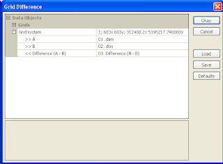
1. Select Modules | Grid | Calculus | Grid Difference.
   
   The Grid Difference dialog box appears.
   
2. In the Grid system field, choose the system of the source datasets, e.g. 683x 683y; 312480x 51952717y.
3. In the A field, choose the digital surface model grid, e.g. dsm.
4. In the B field, choose the digital terrain model grid, e.g. dtm.
5. Click Okay.
   
   The canopy height grid is created.
   

Smooth the canopy heights

1. Select Modules | Grid | Filter | Gaussian Filter.
   
   The Gaussian Filter dialog box appears.
   
2. In the Grid system field, choose the system of the source grid e.g. 683x 683y; 312480x 51952717y.
3. In the Grid field, choose the canopy height grid, e.g. Difference (A-B).
4. In the output Filtered Grid field, choose Create.
5. In the Search Radius field, choose a value to approximate the tree radius e .g. 5.
6. Click Okay.
   
   The smoothed canopy height grid is created.
   

Segment the smoothed canopy heights

1. Select Modules | Imagery | Segmentation | Watershed Segmentation.
   
   The Watershed Segmentation dialog box appears.
   
2. In the Grid system field, choose the grid system of the smoothed grid layer.
3. In the source Grid field, choose the smoothed grid layer e.g. Difference (A-B) [Gaussian Filter].
4. In the Output field, choose Seed.
5. Make sure the Method is set to Maxima.
6. Click Okay.
   
   The canopy heights grid layer is segmented according to maximum heights.
   

Apply a height break limit (removing segments below a certain height)

1. Select Modules | Grid | Calculus | Grid Calculator.
   
   The Grid Calculator dialog box appears.
   
2. In the Grid system field, choose the system of the segmented layer.
3. In the Grids field, click the browse button. In the Grids dialog box that pops up, double click on the segmented  grid layer e.g. "Difference (A-B) [Gaussian Filter][Segments]". Click Okay.
4. In the Formula field, type in the following: ifelse(lt(a,5),-99999,a).
   
   Note: if the grid value is less than 5, then change the grid value to voids (-99999).
5. Click Okay.
   
   The grid layer with no values below the height break limit is created.
   

Convert the segments into vectors

1. Select Modules | Shapes | Grid | Vectorization | Vectorising Grid Classes.
   
   The Vectorising Grid Classed dialog box appears.
   
2. In the Grid system field, choose the system of the previously created grid layer.
3. In the Grid field, choose the grid layer created in the previous step e.g. "Calculation [ifelse(lt(a,5),-99999,a)]".
   
   
   
   
4. Click Okay.
   
   The vector polygon layer is created.
5. Select the shape polygon layer in the Data tab. Then click the Description tab.
   
   The number of shapes shows the approximate count of the number of trees above a height break limit.
   
   
   
   
   The polygons can be displayed as table attribute records as shown below.
   

Simple method to count trees using Saga GIS

It is possible to make a rough estimation of the number of trees in an area from LiDAR derived digital surface (DSM) and digital terrain models (DTM). One method is to use some of the grid analysis modules algorithm in SAGA GIS, such as Gaussian Filter, and Watershed Segmentation. Then simply count the number of segmented table records with height greater than a value.

The example here counts the trees using the following general steps:

1. Load the DSM and DTM datasets
2. Calculate the canopy heights
3. Smooth the canopy heights
4. Segment the canopy heights
5. Count the number of segments with canopy heights above a certain value

Load the source datasets

1. Start SAGA GIS.
2. Load and display the digital surface model (DSM) grid file, e.g. C:\data\dsm.asc.
   
   
   
   
3. Load and display the digital terrain model (DTM) grid file, e.g. C:\data\dtm.asc.
   
   

Calculate the canopy heights

1. Select Modules | Grid | Calculus | Grid Difference.
   
   The Grid Difference dialog box appears.
   
2. In the Grid system field, choose the system of the source datasets, e.g. 683x 683y; 312480x 51952717y.
3. In the A field, choose the digital surface model grid, e.g. dsm.
4. In the B field, choose the digital terrain model grid, e.g. dtm.
5. Click Okay.
   
   The canopy height model grid is created. The default name is Difference(A-B).
   

Smooth the canopy heights

1. Select Modules | Grid | Filter | Gaussian Filter.
   
   The Gaussian Filter dialog box appears.
   
2. In the Grid system field, choose the system of the source grids e.g.  683x 683y; 312480x 51952717y.
3. In the Grid field, choose the canopy height grid, e.g. Difference (A-B).
4. In the output Filtered Grid field, choose Create.
5. In the Search Radius field, choose a value to approximate the tree radius e.g. 5.
6. Click Okay.
   
   The output smoothed grid is created. Default name is Difference (A-B) [Gaussian Filter].
   

Segment the smoothed canopy height model

1. Select Modules | Imagery | Segmentation | Watershed Segmentation.
   
   The Watershed Segmentation dialog box appears.
   
2. In the Grid system field, choose the source grid system e.g.  683x 683y; 312480x 51952717y.
3. In the Grid field, choose the smooth canopy height grid e.g. Difference (A-B) [Gaussian Filter].
4. In the Output field, choose Seed Value.
   
   Note: since the segmentation will be run on the source grid of canopy height values, the resultant seed values will be the estimated heights of the tree tops.
5. Ensure the Method is set to Maxima.
   
   Note: if set to Maxima, the watershed segmentation algorithm will start from the top (max) of the tree and flow down.
6. Optional. Toggle on Borders.
7. Click Okay.
   
   The segmented canopy height grid "Difference (A-B) [Gaussian Filter][Segments]" is created. 
   
   The canopy height point layer "Difference (A-B)[Gaussian Filter][Seed]" is created also.
   

Count the number of segments above a certain canopy height

1. In the Data tree pane, right click on the newly created point layer node under the tree hierarchy - Shapes | Point | 01. Difference (A-B) [Gaussian Filter][Seed].
   
   A pop up menu appears.
2. Choose Attributes | Show.
   
   The attributes table is displayed.
   
3. Right click on the VALUE header.
   
   A pop up menu appears.
4. Choose Sort Fields.
   
   The Sort Table dialog box appears.
   
5. In the Sort first by field, choose VALUE.
6. In the Direction field, choose descending.
7. Click Okay.
   
   The table is sorted.
   
8. Scroll down the table to the rows with the VALUE greater or equal to 5.
   
   The row number on the left indicates the rough estimate of the number of trees greater than 5 meters.
   
   Note: instead of using SAGA GIS to do the counting with the tabular data, it may be easier to export out the point layer into a database software and perform the analysis there. 

Simple canopy height derivation using Global Mapper

The forest canopy height is the height of the highest vegetation above the ground level. It is possible to calculate the canopy height from LiDAR derived digital terrain models (DTM) and digital surface models (DSM) gridded datasets by doing a simple subtraction in Global Mapper. The example below shows how to use the Combine Terrain Layers function in Global Mapper to calculate the canopy height.

1. Start up Global Mapper. Load in a digital terrain model ESRI ArcGrid file e.g. dtm.asc.
   
   
2. Load in a digital surface model ESRI ArcGrid file e.g. dsm.asc.
   
   
3. Select File | Combine Terrain Layers.
   
   The Combine Terrain Options dialog box appears.
   
4. In the Description field, type in relevant text e.g. CanopyHeight.
5. In the Operation field, choose Subtraction (Difference) - Signed.
6. In the Select First Elevation Layer to Combine field, choose the DSM layer e.g. dsm.asc.
7. In the Select Elevation Layer to Combine the First Layer With field, choose the DTM layer e.g. dtm.asc.
   
   
8. Click OK.
9. Press CTRL+C. Toggle off the DTM and DSM layers.
   
   The canopy height is displayed as shown below where the pink indicates zero canopy heights and the blues are positive heights.