Using Saga GIS' Terrain Analysis Swath Profile (interactive) function

Saga GIS has a couple of interactive terrain profiling functions, a single profile and a swath profile. This post shows how to use the interactive swath terrain profile command.

Load a grid file such as a USGS SRTM file

1. Run Saga GIS. Select Geoprocessing | File | Grid | Import | Import USGS SRTM Grid.
   
   The Import USGS SRTM Grid dialog box appears.
   
2. Click the Browse button in the Files field. Choose an SRTM file e.g. N21E093.hgt.
   
   
3. Click Open.
   
   
4. Click Okay.
   
   The SRTM file is loaded and shown in the Data tab.
   

Start the swath profile command

1.  Under the Data tab, mouse right click on the loaded grid file e.g. N21E093.
2. In the pop up context menu, choose Add to Map.
   
   The grid file is displayed in a map window.
   
3. Select Geoprocessing | Terrain Analysis | Profiles | Swath Profle [Interactive].
   
   The Swath Profile dialog box appears.
   
4. In the Grid system field, choose the loaded grid file's system e.g. 0.000833; 1201x 1201y; 93x 21y option.
5. In the DEM field, choose the loaded grid file, e.g. N21E093.
6. Optional. Change the Swath Width if necessary.
   
   The message Interactive tool execution has been started is displayed in the Messages pane.

Digitize the swath profile

1. In the Toolbar, click the Action icon (that looks like a black NW arrow).
2. In the map window, click a few points to draw the swath profile.
   
   
   
3. To complete the drawing, press the mouse right button.
4. To exit the interactive command, select Geoprocessing | Swath Profle [Interactive].
   
   The Tool Execution prompt appears.
   
5. Click Yes.
   
   The message: "Interactive tool execution has been stopped" is shown in the Messages pane.
   
   Note: This may take a while as the command will sample the terrain to calculate the points.

Display the swath profile graphically

1.  In the Data pane, mouse right click on the newly created profile points e.g. Profile [N21E093].
   
   
2. In the pop up menu, choose Attributes | Diagram.
   
   The Properties dialog box appear.
   
3. In the X Axis Values field, choose D (for Distance).
4. In the X Axis Label field, choose D.
5. In the Attributes field, toggle on Z, Z [min], Z[max].
6. Set other options if necessary.
7. Click Okay.
   
   The profile line(s) are displayed.
   

Create a Facebook 3D Photo of a digital elevation model using QGIS

Facebook has a 3D photo feature which brings perspective and movement to the Facebook news feed and timeline images. A live example can be seen embedded here:


Normally these images are created using RGB-D cameras, where D stands for depth. However it is also possible to workaround it without a RGB-D camera by uploading to Facebook two images - an RGB image and its corresponding grayscale depth image, and making sure the depth image has the same name as the RGB image with a '_depth' suffix. The depth image is grayscale only with values ranging from dark to light -  the dark pixels representing the furthest pixels and the light pixels representing the nearest pixels.

Using the ideas above, the following steps illustrate how to create a Facebook 3D Photo image from a SRTM digital elevation model (DEM) using QGIS.

1. Startup QGIS. Create a new project. If the canvas background is not already black, select Project | Project Properties.
   
   The Project Properties dialog box appears.
   
2. In the Background color field, change the color to black. Click OK.
   
   The canvas background becomes black.
   
3. Drag and drop a DEM file onto the canvas e.g. srtm_54_07.tif.
   
    
4.  Optional. To serve the purpose of having a background, an OpenStreetMap (OSM) layer is displayed behind the DEM layer.
   
   
5. Optional. To display only DEM heights above an elevation of interest, e.g. 200 meters, right click on the DEM layer and choose Properties. Then add in a new transparent entry to the transparent pixel list from 0 to 200 meters, as shown below. Then click OK.
   
   The Layer Properties dialog box appears.
   
   
   
   The DEM display is updated.
   
   
6. Make a duplicate of the DEM layer by right clicking on the DEM layer and choosing Duplicate. Rename the copy as 'depth' as it will serve to generate a depth image later on.
   
   
7. Right click on the top most DEM layer and choose Properties. In the Layer properties dialog box, click Style.
   
   
8. Change the Render Type to Hillshade. Click OK.
   
   The DEM layer is now rendered as a hill shade.
   
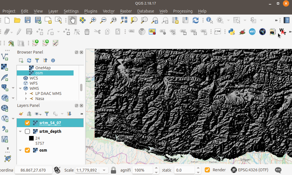
9. Make a duplicate copy of the hill shaded DEM layer by right clicking the layer and choosing Duplicate. Rename the copy as 'hillshade' as shown below.
   
   
10. Right click on the top most DEM layer and choose Properties. Select the Style tab.
    
    
11. In the Rendering type field, choose Singleband pseudocolor. Choose a suitable color gradient e.g. Spectral and toggle Invert if necessary. Choose a suitable Blending mode e.g. Screen.
    
    
12. Click OK.
    
    The DEM layer is rendered with a colored gradient.
    
13. With the gradient colored, hill shaded and OSM layers displayed on and the depth layer displayed off, export out the canvas by selecting Project | Save as image and specifying an output file name e.g. srtm.png.
    
    The srtm image is generated.
    
14. Now turn off the gradient, hill shaded and OSM layers. Turn on the depth layer as shown below.
    
    
    
    
    Select Project | Save as image to export out the depth image with a '_depth' suffix e.g. srtm_depth.png.
    
    The srtm_depth image is generated.
    
15. Now open up Facebook in a browser and click the Post Photo/Video button.
    
    The File Upload dialog box appears.
    
16. Browse and select the generated srtm.png and srtm_depth.png files. Click Open.
    
    Facebook generates the 3D Photo.
    
    
    A live example is available here at https://www.facebook.com/permalink.php?story_fbid=1251984134967474&id=101193703379862