C# code snippet to determine if a point is in a polygon

A common test in GIS is to determine whether a point is inside a polygon or not.
The following C# code snippet can determine whether a point is inside a simple 2-D polygon. Just pass in an array of the polygon vertices and the point. The function returns true if the point is in the polygon and false if it is not.

private bool IsPointInPolygon(PointF[] polygon, PointF point)

{

bool isInside = false;

for (int i = 0, j = polygon.Length - 1; i < polygon.Length; j = i++)

{

if (((polygon[i].Y > point.Y) != (polygon[j].Y > point.Y)) &&

(point.X < (polygon[j].X - polygon[i].X) * (point.Y - polygon[i].Y) / (polygon[j].Y - polygon[i].Y) + polygon[i].X))

{

isInside = !isInside;

}

}

return isInside;

}

Simple method to count trees using Saga GIS

It is possible to make a rough estimation of the number of trees in an area from LiDAR derived digital surface (DSM) and digital terrain models (DTM). One method is to use some of the grid analysis modules algorithm in SAGA GIS, such as Gaussian Filter, and Watershed Segmentation. Then simply count the number of segmented table records with height greater than a value.

The example here counts the trees using the following general steps:

1. Load the DSM and DTM datasets
2. Calculate the canopy heights
3. Smooth the canopy heights
4. Segment the canopy heights
5. Count the number of segments with canopy heights above a certain value

Load the source datasets

1. Start SAGA GIS.
2. Load and display the digital surface model (DSM) grid file, e.g. C:\data\dsm.asc.
   
   
   
   
3. Load and display the digital terrain model (DTM) grid file, e.g. C:\data\dtm.asc.
   
   

Calculate the canopy heights

1. Select Modules | Grid | Calculus | Grid Difference.
   
   The Grid Difference dialog box appears.
   
2. In the Grid system field, choose the system of the source datasets, e.g. 683x 683y; 312480x 51952717y.
3. In the A field, choose the digital surface model grid, e.g. dsm.
4. In the B field, choose the digital terrain model grid, e.g. dtm.
5. Click Okay.
   
   The canopy height model grid is created. The default name is Difference(A-B).
   

Smooth the canopy heights

1. Select Modules | Grid | Filter | Gaussian Filter.
   
   The Gaussian Filter dialog box appears.
   
2. In the Grid system field, choose the system of the source grids e.g.  683x 683y; 312480x 51952717y.
3. In the Grid field, choose the canopy height grid, e.g. Difference (A-B).
4. In the output Filtered Grid field, choose Create.
5. In the Search Radius field, choose a value to approximate the tree radius e.g. 5.
6. Click Okay.
   
   The output smoothed grid is created. Default name is Difference (A-B) [Gaussian Filter].
   

Segment the smoothed canopy height model

1. Select Modules | Imagery | Segmentation | Watershed Segmentation.
   
   The Watershed Segmentation dialog box appears.
   
2. In the Grid system field, choose the source grid system e.g.  683x 683y; 312480x 51952717y.
3. In the Grid field, choose the smooth canopy height grid e.g. Difference (A-B) [Gaussian Filter].
4. In the Output field, choose Seed Value.
   
   Note: since the segmentation will be run on the source grid of canopy height values, the resultant seed values will be the estimated heights of the tree tops.
5. Ensure the Method is set to Maxima.
   
   Note: if set to Maxima, the watershed segmentation algorithm will start from the top (max) of the tree and flow down.
6. Optional. Toggle on Borders.
7. Click Okay.
   
   The segmented canopy height grid "Difference (A-B) [Gaussian Filter][Segments]" is created. 
   
   The canopy height point layer "Difference (A-B)[Gaussian Filter][Seed]" is created also.
   

Count the number of segments above a certain canopy height

1. In the Data tree pane, right click on the newly created point layer node under the tree hierarchy - Shapes | Point | 01. Difference (A-B) [Gaussian Filter][Seed].
   
   A pop up menu appears.
2. Choose Attributes | Show.
   
   The attributes table is displayed.
   
3. Right click on the VALUE header.
   
   A pop up menu appears.
4. Choose Sort Fields.
   
   The Sort Table dialog box appears.
   
5. In the Sort first by field, choose VALUE.
6. In the Direction field, choose descending.
7. Click Okay.
   
   The table is sorted.
   
8. Scroll down the table to the rows with the VALUE greater or equal to 5.
   
   The row number on the left indicates the rough estimate of the number of trees greater than 5 meters.
   
   Note: instead of using SAGA GIS to do the counting with the tabular data, it may be easier to export out the point layer into a database software and perform the analysis there. 

Simple canopy height derivation using Global Mapper

The forest canopy height is the height of the highest vegetation above the ground level. It is possible to calculate the canopy height from LiDAR derived digital terrain models (DTM) and digital surface models (DSM) gridded datasets by doing a simple subtraction in Global Mapper. The example below shows how to use the Combine Terrain Layers function in Global Mapper to calculate the canopy height.

1. Start up Global Mapper. Load in a digital terrain model ESRI ArcGrid file e.g. dtm.asc.
   
   
2. Load in a digital surface model ESRI ArcGrid file e.g. dsm.asc.
   
   
3. Select File | Combine Terrain Layers.
   
   The Combine Terrain Options dialog box appears.
   
4. In the Description field, type in relevant text e.g. CanopyHeight.
5. In the Operation field, choose Subtraction (Difference) - Signed.
6. In the Select First Elevation Layer to Combine field, choose the DSM layer e.g. dsm.asc.
7. In the Select Elevation Layer to Combine the First Layer With field, choose the DTM layer e.g. dtm.asc.
   
   
8. Click OK.
9. Press CTRL+C. Toggle off the DTM and DSM layers.
   
   The canopy height is displayed as shown below where the pink indicates zero canopy heights and the blues are positive heights. 
   

Google Mapplet for State Plane Coordinate System readout

The State Plane Coordinate System (SPCS) is a map coordinate system commonly used in the United States. Most SPCS zones are based on the Transverse Mercator, Lambert Conformal Conic or Hotine Oblique Mercator projections. For more information about SPCS, visit this site at http://en.wikipedia.org/wiki/State_Plane_Coordinate_System.

This Google Mapplet can be used to display any State Plane Coordinate System coordinates. You do have to choose which coordinate system to use e.g. Alabama East Zone FIPS101 and the NAD83 datum. Then simply click anywhere on the map and the mapplet will display the SPCS easting, northing coordinates as shown below.

The datum transformation between the WGS84 datum used by Google Maps and the local NAD27 or NAD83 projection datum is done using the Standard Molodensky transformation. Parameters for the datums and ellipsoids are taken from the University of Colorado.

Click this link http://dominoc925-pages.appspot.com/mapplets/cs_spcs.html to run the mapplet.

Google Mapplet for showing UTM grid zones

The Universal Transverse Mercator (UTM) coordinate system is a grid based system for specifying locations on the earth's surface. UTM consists of 60 zones, each with its own local Transverse Mercator projection. The Wikipedia site http://en.wikipedia.org/wiki/Universal_Transverse_Mercator_coordinate_system has more information about UTM.

This Google Mapplet was created to display the UTM grid zones and labels on interactive maps. The current version allows the user to change the grid line color for better visualization over different backdrops.

Click this link http://dominoc925-pages.appspot.com/mapplets/utmgrid.html to run the mapplet.

Join a spatial table with a non-graphical table in gvSIG

It is very useful to join a geospatial feature with a related non-graphical database table for analysis. This is a common feature found in commercial GIS applications like GeoMedia. I found a similar function in the open-source software gvSIG although it seems to handle only inner type joins. An example of using the gvSIG Join command is described below.

1. Start gvSIG OADE. Load and display a geospatial feature e.g. States.shp in a map view.
    
2. Load a database table e.g. SalesByStates.dbf.
   
   
   
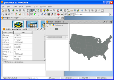
3. In the Map view legend TOC, click on the geospatial feature name e.g. States.shp. Then press the right button of the mouse on the name.
   
   A pop up menu appears.
   
4. Choose Join.
   
   The Join tables dialog box appears.
   
   
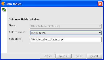
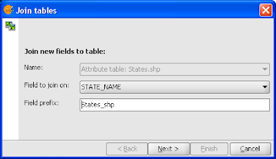
5. In the Field to join on combo box, choose a common field between the graphical and non-graphical table e.g. STATE_NAME.
   
6. In the Field prefix field, type in the prefix string to indicate the fields from the geospatial feature table e.g. States_shp. Click Next.
   
   
   
7. In the Name field, choose the non-graphical table e.g. SalesByStates.dbf.
   
8. In the Field to join on, choose the common field between the non-graphical table and the feature table e.g. STATE_NAME.
   
9. In the Field prefix field, type in the prefix string to indicate the fields from the non-graphical table e.g. SalesByStates_dbf. Click Finish.
   
   
   
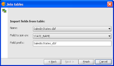
   The tables are joined.

To see the results of the join, you can view the attribute table or query the attributes of selected features. For example, press CTRL+I, then click on any feature in the map view. The Query results dialog box should appear showing the joined table attributes, as shown below.

Connect to non-graphical tabular database data in gvSIG

Being used to commercial GIS software, I was looking around for the option to connect to a non-graphical database table in the gvSIG OADE 2010 application window. I failed to locate the command. Later on, I saw that the command is contained in the Project Manager window - a child form within the main gvSIG application window. Once I found it, it was quite easy to connect to the non-graphical database table as shown in the dbf example below.

1. Start up gvSIG OADE 2010.
2. In the Project Manager dialog box, click the Table button.
   
   
3. Click the New button.
   
   The New table dialog box appears.
   
4. Click Add.
   
   The Open dialog box appears.
   
5. Browse and select a dbf file e.g. SalesByState.dbf. Click Open.
   
   The selected file is added to the list of Tables.
   
6. Click OK.
   
   The attribute table is displayed in gvSIG.